In Google Sheets, we may use the VLOOKUP function to look up a particular value from our dataset. Since, the VLOOKUP function has some disadvantages, like if we insert a column in our dataset, the result might change because of this. So, we can use an alternative to the VLOOKUP function in Google Sheets to get a similar outcome. In this article, I will show 8 easy alternative to the VLOOKUP function in Google Sheets.
8 Alternative Methods to Use VLOOKUP Function in Google Sheets
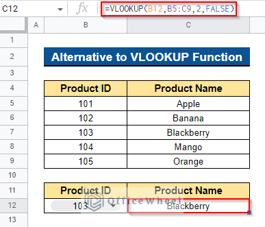
We will use the dataset below to demonstrate the examples of 8 easy alternative to the VLOOKUP function in Google Sheets. The dataset contains the Product ID and Product Name of a shop. We have used a VLOOKUP formula in Cell C12 to look up the value of a Product Name based on the Product ID on Cell B12. Now, we will use the alternative of the VLOOKUP function to get a similar result.
1. Using XLOOKUP Function
The ideal replacement for the VLOOKUP Function is the XLOOKUP function. Using the XLOOKUP function, you can look up a value in any row or column and then get the value of a cell that matches that search term from a different row or column. By default, the XLOOKUP function can locate exact matches. It can search in any direction. The XLOOKUP function allows you to return a range of values. Using this function, you may search across a number of criteria. You can add, update, or remove columns using the XLOOKUP function.
Steps:
- First, select a cell where you want to apply the formula. In our case, we selected Cell C12.
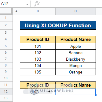
- Now, type the formula below and press the Enter button-
=XLOOKUP(B12,B5:B9,C5:C9)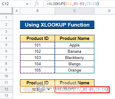
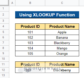
- Then, it will display the Product Name based on the Product ID on Cell B12.
Read More: How to VLOOKUP for Partial Match in Google Sheets
2. Combining INDEX and MATCH Functions
The most popular substitute for the VLOOKUP Function in Google Sheets is the combination of the INDEX and MATCH functions. The input for the lookup column is made using the MATCH function, which also does the search. While the INDEX function uses the return column to return a value that matches the output of the MATCH function.
2.1 For Single Criteria
We can look up a value in Google Sheets using the combination of the INDEX and MATCH functions based on single criteria.
Steps:
- First, choose the cell to which you wish to apply the formula. We chose Cell C12. Now, enter the formula below and hit Enter–
=INDEX(C5:C9,MATCH(B12,B5:B9,0))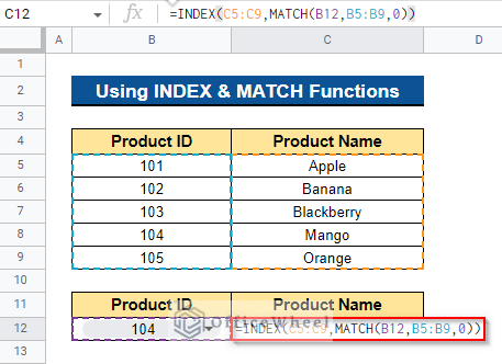
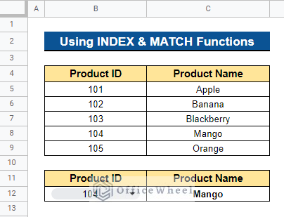
- Then, depending on the Product ID in Cell B12, it will show the Product Name.
Read More: Combine VLOOKUP and HLOOKUP Functions in Google Sheets
2.2 For Multiple Criteria
Sometimes we want to look up a value in Google Sheets based on multiple criteria. We can easily do this by combining the INDEX and MATCH functions.
Steps:
- We want to look up the value of the Sales based on the Product ID on Cell B12 and the Shop on Cell C12. To do this, first select a cell where you will apply the formula. Then type the formula below and hit Enter–
=INDEX(D5:D9,MATCH(1,(B5:B9=B12)*(C5:C9=C12),0))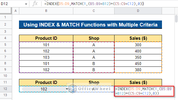
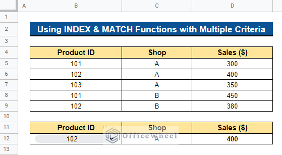
Like the previous breakdown, the MATCH function will return the relative position for the multiple criteria and then the INDEX function will return the output according to the relative position.
- Thus, you will get the value of the Sales whose Product ID is 102 and which is from Shop A.
Read More: Find All Cells With Value in Google Sheets (An Easy Guide)
3. Merging OFFSET and MATCH Functions
The combination of the OFFSET and MATCH functions in Google Sheets, which functions similarly to the combination of the INDEX & MATCH functions, is another alternative to the VLOOKUP function.
Steps:
- To apply the formula, choose the cell where it should go. We chose Cell C12 in our case. Press the Enter key after typing the formula below-
=OFFSET(B4,MATCH(B12,B5:B9,0),MATCH(C11,C4))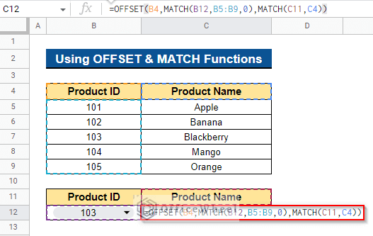
Formula Breakdown
- MATCH(B12,B5:B9,0)
First, it will return the relative location of Cell B12 in a range of Cell B5:B9.
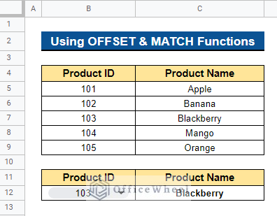
- OFFSET(B4,MATCH(B12,B5:B9,0),MATCH(C11,C4))
Then a range reference that has been moved by the provided number of rows and columns from the beginning cell reference will be returned.
- Thus, using the Product ID in Cell B12 as a basis, it will display the Product Name.
Similar Readings
- Use of Google Sheets INDEX MATCH in Multiple Columns
- How to Create Conditional Drop Down List in Google Sheets
- Google Sheets Vlookup Dynamic Range
- How to VLOOKUP All Matches in Google Sheets (2 Approaches)
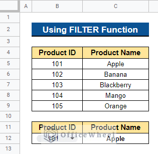
4. Using FILTER Function
The FILTER function in Google Sheets is an additional substitute for the VLOOKUP function. It is one of the quicker options to utilize.
Steps:
- First, choose a cell to which you will first apply the formula. In this instance, we chose Cell C12. Enter the formula below and then click Enter.
=FILTER(C5:C9,B5:B9=B12)
- You will get your desired result.
Read More: How to VLOOKUP Left in Google Sheets (4 Simple Ways)
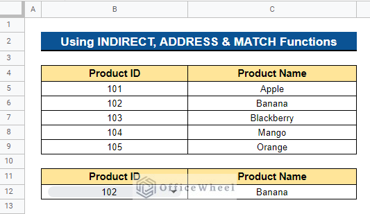
5. Associating INDIRECT, ADDRESS, and MATCH Functions
The combination of the INDIRECT, ADDRESS and MATCH functions is another substitute for the VLOOKUP function in Google Sheets. However, in order to utilize this choice, you must start from the first cell in a column or row.
Steps:
- First, choose the cell to which you wish to apply the formula. We chose Cell C12. Now, enter the formula below and hit the Enter
=INDIRECT(ADDRESS(MATCH(B12,B1:B9,0),MATCH(C11,A4:C4,0)))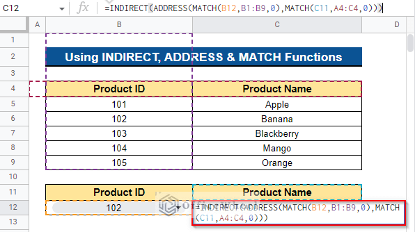
Formula Breakdown
- MATCH(B12,B5:B9,0)
First, the relative position of Cell B12 in the range of Cell B5:B9 will be returned.
- ADDRESS(MATCH(B12,B1:B9,0),MATCH(C11,A4:C4,0))
A string containing a cell reference will be returned.
- INDIRECT(ADDRESS(MATCH(B12,B1:B9,0),MATCH(C11,A4:C4,0)))
Then the INDIRECT function will return the cell reference designated via the string.
- Thus, you will get the output of the Product Name based on the Product ID on Cell B12.
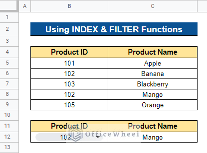
6. Coupling INDEX and FILTER Functions to Show Nth Match
We might occasionally need to search Google Sheets for the Nth match in the dataset. We can accomplish this by using the combination of the INDEX and FILTER functions.
Steps:
- For a single Product ID, we have two Product Names. Additionally, we want to check for the Product Name‘s second value. To do this, first select a cell. We selected Cell C12. Now enter the following formula into the cell and press the Enter key-
=INDEX(FILTER(C5:C9,B5:B9=B12),2)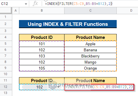
Formula Breakdown
- FILTER(C5:C9,B5:B9=B12)
First, only the rows or columns that satisfy the defined criteria will be returned in the filtered form of the source range.
- INDEX(FILTER(C5:C9,B5:B9=B12),2)
Then the INDEX function will return the 2nd value of the Product Name specified by FILTER(C5:C9,B5:B9=B12).
- As a result, based on Cell B12, it will display the second value of the Product Name for the Product ID.
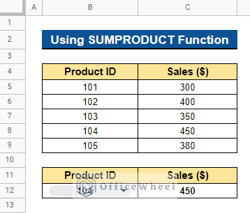
7. Applying SUMPRODUCT Function
If we need to look up numbers, the SUMPRODUCT function is a viable alternative to the VLOOKUP function. The ease of applying numerous criteria is one benefit of the SUMPRODUCT function.
Steps:
- To apply the formula, first select a cell. We selected Cell C12. Now type the formula below and hit Enter.
=SUMPRODUCT((B5:B9=B12)*C5:C9)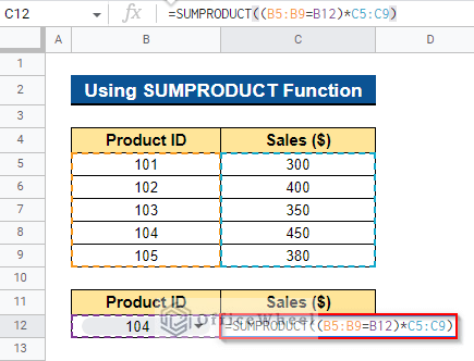
- Thus, you will get the desired output in your desired cell.
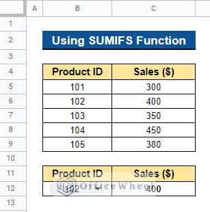
8. Employing SUMIFS Function
Instead of utilizing the SUMPRODUCT Function, we may use the SUMIFS function to search for numbers based on a variety of criteria. The SUMIFS function is easier and more straightforward to use.
Steps:
- To begin, select a cell where you want to apply the formula. We selected Cell C12. Now, type the formula below and press Enter-
=SUMIFS(C5:C9,B5:B9,B12)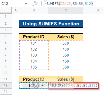
- Thus, you will get the Sales of the product based on the Product ID on Cell B12.
Conclusion
In this article, I have shown 8 easy alternatives to the VLOOKUP function in Google Sheets. You can use any of the alternatives and you will get a similar result. Furthermore, I have shown how to use the combination of the INDEX and MATCH functions for multiple criteria in Google Sheets. Please feel free to ask any questions or suggest any ideas. Visit officewheel.com to explore more.
Related Articles
- [Fixed!] INDEX MATCH Is Not Working in Google Sheets (5 Fixes)
- Google Sheets Conditional Formatting with INDEX-MATCH
- Match Multiple Values in Google Sheets (An Easy Guide)
- Find Cell Reference in Google Sheets (2 Ways)
- How to Use VLOOKUP with Named Range in Google Sheets
- How to Check If Value Exists in Range in Google Sheets (4 Ways)
- How to Do Reverse VLOOKUP in Google Sheets (4 Useful Ways)
- How to Use VLOOKUP to Import from Another Workbook in Google Sheets