VLOOKUP is a powerful function in Google Sheets for finding data in large tables. It is widely used by businesses and individuals to simplify data management and analysis tasks. The dynamic VLOOKUP is an advanced version of the standard VLOOKUP, offering even more versatility and flexibility to users. In this article, we will explore the benefits of using Google Sheets dynamic range VLOOKUP and learn how to implement it in your next project.

Problem with Regular VLOOKUP Function in Google Sheets and Why is Having a Dynamic Range Necessary?
The regular VLOOKUP function in Google Sheets has two main limitations: it can only search for values in the first column of the lookup table, and it cannot automatically adjust the lookup range when data is added or deleted from the table.
Syntax:
VLOOKUP(search_key, range, index, [is_sorted])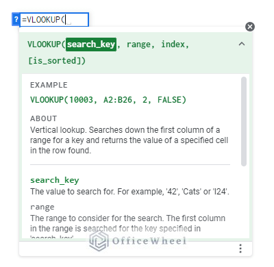
- “Search key,” the first argument, defines the value to look for in the first column of the given range.
- “range“, the second argument, defines the table or range of cells to search within.
- The third argument, “index“, indicates the column number within the range to return the matching value.
- The final and fourth argument is “is_sorted” which determines whether the first column of the range is sorted in ascending order. If the first column is sorted, set “is_sorted” to TRUE, otherwise set it to FALSE.
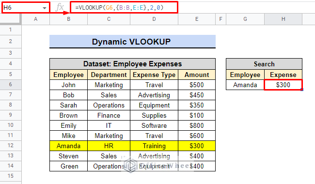
Check the following images for example.
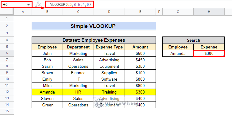
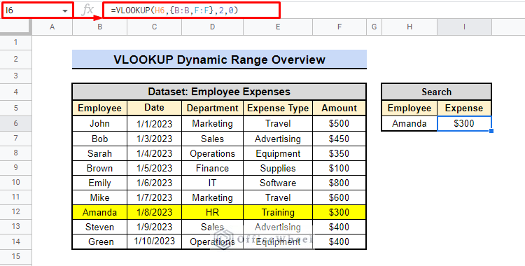
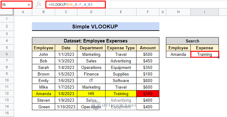
We have a database of expenses made by employees and we want to determine the amount spent by Amanda. A simple VLOOKUP can easily retrieve this information, but the date of the expenses is not included in the dataset. Adding a date column could alter the results of the VLOOKUP.
Having a dynamic range with VLOOKUP overcomes these limitations, as it allows for searching in any column and automatically adjusts the lookup range. This results in more flexible and efficient data lookups.
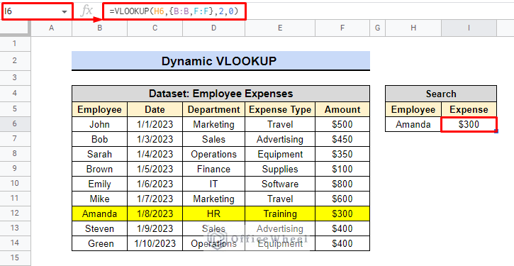
As an example, we used the same dataset. But in this instance, including a new date column has no impact on the outcome. Instead, it changed the range for columns E to F. Observing the formula makes it simple to see the shift.
Therefore, it is clear that VLOOKUP dynamic range is quite beneficial in google sheets when used professionally.
2 Simple Approaches to Apply Dynamic Range in VLOOKUP in Google Sheets
Dynamic range in VLOOKUP is a valuable feature in Google Sheets that helps ensure the accuracy and efficiency of your data analysis. With dynamic range, the VLOOKUP formula automatically adjusts to match the size of the data range.
This article will explore two simple approaches to applying dynamic range in VLOOKUP in Google Sheets.
1. Implementing VLOOKUP Field Values as Array in Same Worksheet
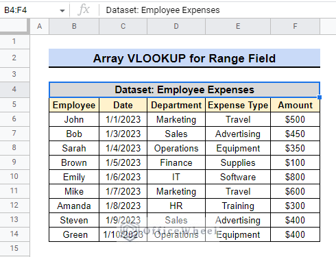
Assume that we have a financial database that showcases the employee expenses incurred during their business trips.
I. For Range Field
Consider that we want to determine the type of expense and department by using the employee name as the lookup value and using the dynamic VLOOKUP feature.
Steps:
- Firstly, we will select cell I6.
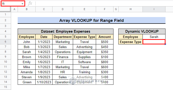
- Secondly, we will use the following formula to find the expense type by the employee.
=VLOOKUP(H6,{B:B,E:E,D:D},2,0)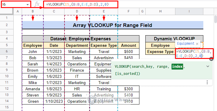
- The curly braces {} in the VLOOKUP formula allow you to select multiple columns in any order, unlike the normal VLOOKUP using parentheses () which follows a sequential order.
- For example, in the formula, columns B, E, and D are selected using curly braces in an order that can benefit us.
- The difference between using curly braces and parentheses in VLOOKUP can impact the results of the calculation, so it’s important to understand when to use each.
- Finally, press ENTER to see the result.
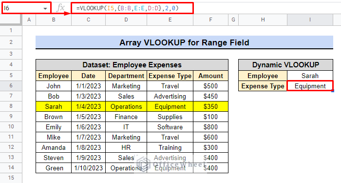
- The formula will return the value in the second column (column index 2) of the matching row that contains the lookup value in column E.
We can also get the department just by changing the column index from 2 to 3.
=VLOOKUP(I5,{B:B,E:E,D:D},3,0)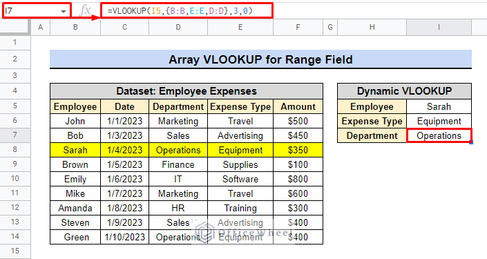
By adjusting the index number, we can specify which column in the matching row to return the value from. For instance, we used the same formula to retrieve the department name.
Read More: How to Use VLOOKUP with Named Range in Google Sheets
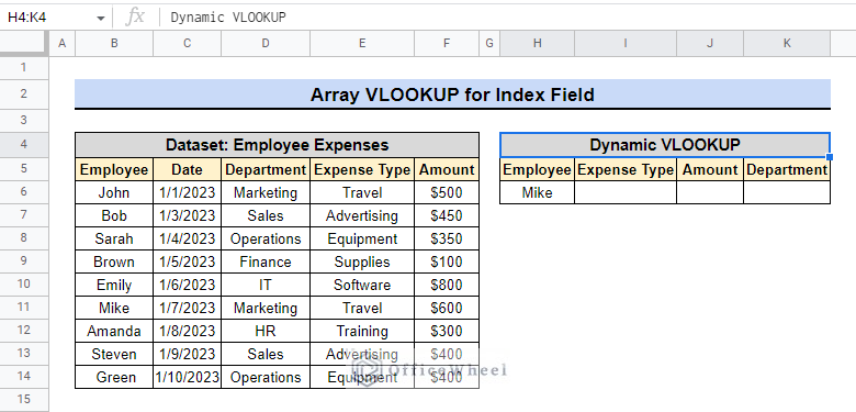
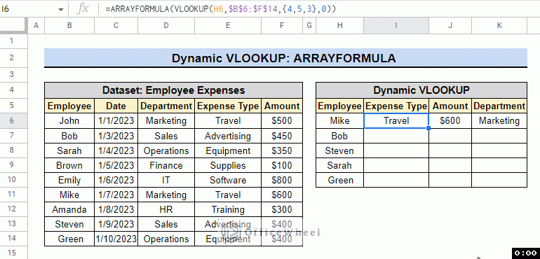
II. For Index Field (Getting Multiple Results with VLOOKUP Dynamically)
We will use the same dataset, but this time we will retrieve all the relevant information in one go. For instance, we will search by the employee name and retrieve the type of expense, the amount of the expense, and the name of the department.
Steps:
- Once again we will select cell I6 first.
- Now, we will use the following formula.
=ARRAYFORMULA(VLOOKUP(H6,$B$6:$F$14,{4,5,3},0))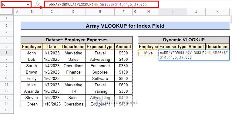
- Finally, pressing the ENTER key will display all the relevant results.
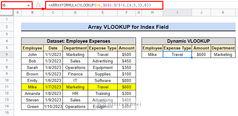
- The first argument for the VLOOKUP function is “H6” as a search key.
- Second argument for the VLOOKUP function is “$B$6:$F$14“, which refers to the data range being searched.
- The third argument is “{4,5,3}“, which tells the formula to return the values in columns 4, 2, and 5 for the matching row.
- The final argument for the VLOOKUP function is “0“, which means that an exact match must be found in the data range for the formula to return a result.
- Finally, ARRAYFORMULA enables the formula to return a result over a range of cells.
The use of ARRAYFORMULA in dynamic VLOOKUP has the benefit of allowing you to return multiple results from multiple columns at once. This saves time and effort compared to having to use multiple individual VLOOKUP formulas.
Read More: How to VLOOKUP Multiple Columns in Google Sheets (3 Ways)
2. Using Functions to Create Dynamic Range from Different Worksheets
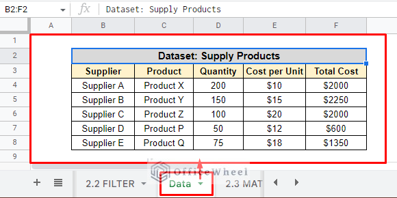
We will use two new datasets. One is about supplies and their quantities and costs and another is about toy store products. These data are in a different sheet or spreadsheet. The following methods will help us understand how to access it.
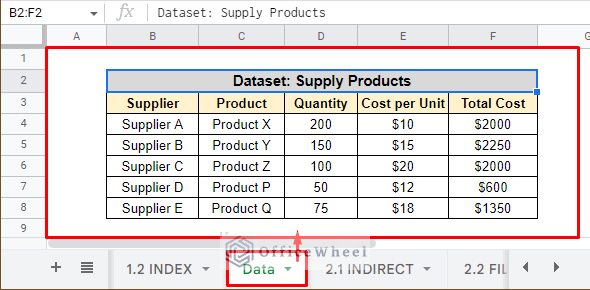
Consider that we will use the product supply data in the Datasheet to illustrate these methods.
I. Using INDIRECT Function for VLOOKUP Range
The INDIRECT function combined with VLOOKUP allows for dynamic referencing of data, making it easy to update VLOOKUP formulas as data changes. This saves time and effort by eliminating the need to manually adjust formulas every time the source data changes.
Syntax:
INDIRECT(cell_reference_as_string, [is_A1_notation])Assume that we’ll use the INDIRECT function to find the total cost of products supplied by Suppliers C, E, and B. The data is on a separate sheet called “Data” and will be used as a cell reference.
Steps:
- At first, we will select cell C6.
- Then, we will apply the following formula.
=VLOOKUP(B8,INDIRECT("'"&B$4&"'!"&"B4:F13"),5)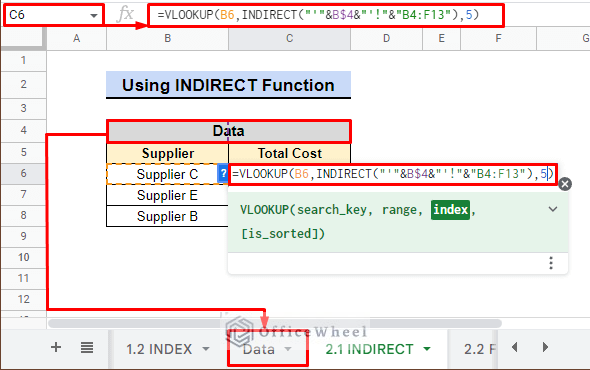
- The VLOOKUP function searches for a value (B8) in the first column of a specified range table array.
- Generally, the INDIRECT function creates a dynamic cell reference to a specific sheet and range, in this case, the “Data” sheet and B4:F13 range.
- The 5 in the VLOOKUP formula indicates which column from the specified range will be returned as a result.
- The formula returns the value from the fifth column of the specified range where the value in B8 is found in the first column.
- Finally, press ENTER to see the total cost of the product supplied by Supplier C.
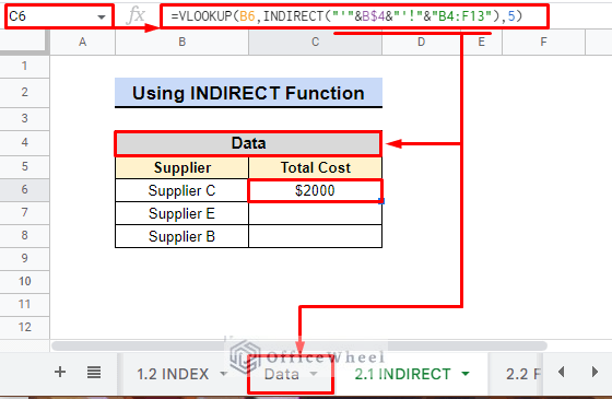
- The formula allows us to search for data outside the current sheet. It helps to determine the total cost for Suppliers E and B with ease.
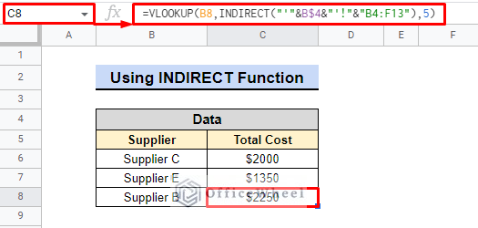
It is evident that instead of manually copying data from one sheet to another, we can simply use the INDIRECT and VLOOKUP formulas to reference the data and automatically retrieve it.
Read More: Combine VLOOKUP and HLOOKUP Functions in Google Sheets
Similar Article
- How to VLOOKUP Between Two Google Sheets (2 Ideal Examples)
- Create Hyperlink to VLOOKUP Cell in Multiple Rows in Google Sheets
- How to Concatenate with VLOOKUP in Google Sheets
- 2 Helpful Examples to VLOOKUP by Date in Google Sheets
- How to Use VLOOKUP Function for Exact Match in Google Sheets
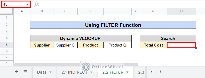
II. Using FILTER Function
Using the VLOOKUP function, we can not only search for data but also filter it by combining it with the FILTER function. Let’s take an example where we want to find the total cost of Product Q supplied by Supplier C.
Syntax:
FILTER(range, condition1, [condition2, ...])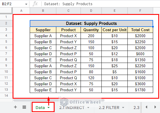
The FILTER function allows us to easily find specific products from Supplier C, which supplies both Product Q and Product Z.
Steps:
- Firstly, We will select cell C6.
- Secondly, we will use the following formula to filter data.
=VLOOKUP(C5,FILTER(Data!B:F,Data!C:C=E5),5,0)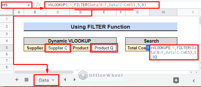
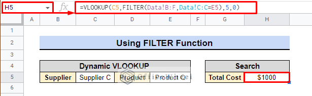
- In the end, press ENTER to see the total cost.
- C5 is the lookup value to be searched for in the data range.
- FILTER(Data!B:F,Data!C:C=E5) returns a filtered data range from the “Data” sheet, where the values in column C match the value in cell E5.
- 5 is the column number of the data range to return the result.
- 0 indicates an exact match is required for the lookup value.
- The above image shows us that we used the FILTER function along with VLOOKUP to filter data and find the total cost of Product Q supplied by Supplier C, which is $2000.
The combination of FILTER and VLOOKUP allows us to quickly and efficiently find specific information from large data sets.
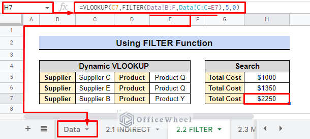
By using this combination, we provided multiple examples such as, we find the total cost for Product Y supplied by Supplier B, and can easily extend the search for other suppliers and products.
Read More: Alternative to Use VLOOKUP Function in Google Sheets
III. Using MATCH Function for Dynamic Column Number
The use of the MATCH function as a column index in the VLOOKUP dynamic range offers two benefits: improved accuracy and flexibility in data retrieval.
Syntax:
MATCH(search_key, range, [search_type])It allows us to select the exact column we want to retrieve data from, eliminating the need for manual updates to our formulas when the structure of our data changes.
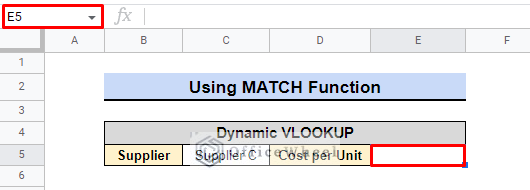
Assume that we are going to find the cost per unit for the product supplied by supplier C.
Steps:
- Once again, we will select cell E5.
- Now, we will use the following formula
=VLOOKUP(C5,Data!B:F,MATCH(D5,Data!$B$3:$3,0),0)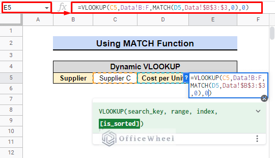
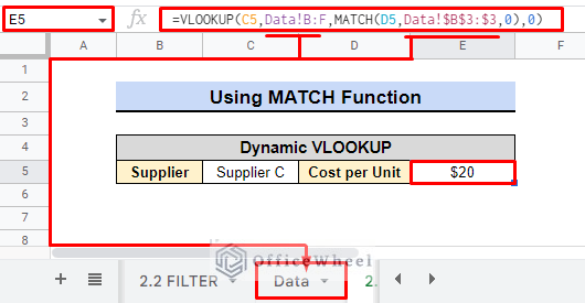
- Finally, press ENTER to see the result.
- Firstly, the VLOOKUP formula takes the value in cell E5 as the lookup value.
- Secondly, it references the data range in the “Data” sheet from column B to column F.
- Next, it uses the MATCH function to find the column index where the header value in cell D5 is found in the range Data!$B$3:$3.
- Finally, the VLOOKUP formula returns the value in the same row as the lookup value and in the column found by the MATCH function, with an exact match (0) setting.
The output is $20 which means that the cost per unit for the product supplied by Supplier C is $20.
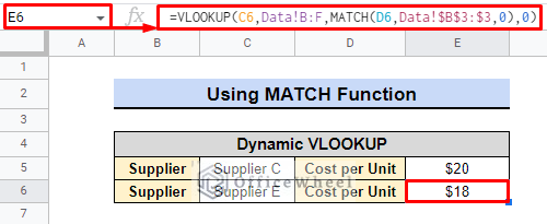
By combining the power of FILTER and VLOOKUP, we are able to effortlessly uncover valuable information from our data. The formula helps us find the cost per unit for a specific supplier, like Supplier E which is $18.
Read More: How to VLOOKUP Last Match in Google Sheets (5 Simple Ways)
IV. Using IMPORTRANGE Function
The IMPORTRANGE function in Google Sheets allows us to easily retrieve data from another spreadsheet.
Syntax:
IMPORTRANGE(spreadsheet_url, range_string)In this example, we have a dataset of a toy store’s products and we want to find out how many are in stock using the product ID. The link to the dataset is as follows.
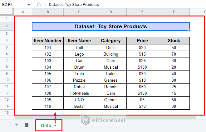
Steps:
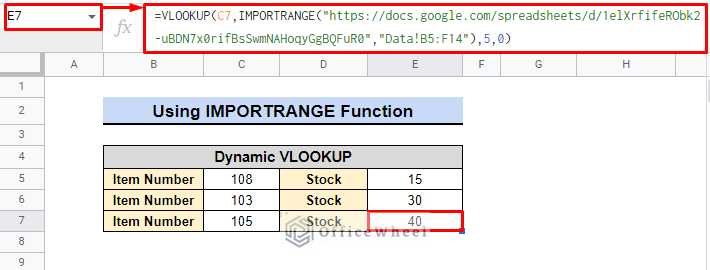
- First, we will select cell E5.
- Second, we’ll input the formula:
=VLOOKUP(C5,IMPORTRANGE("https://docs.google.com/spreadsheets/d/1elXrfifeRObk2-uBDN7x0rifBsSwmNAHoqyGgBQFuR0","Data!B5:F14"),5,0)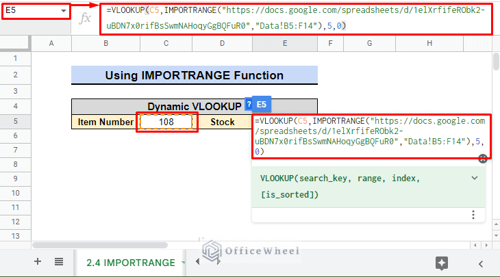
- C5 is the search key for the product ID we want to look up.
- IMPORTRANGE(“https://docs.google.com/spreadsheets/d/1elXrfifeRObk2-uBDN7x0rifBsSwmNAHoqyGgBQFuR0″,”Data!B5:F14”) retrieves the data from another spreadsheet.
- 5 is the index number, representing the column we want to retrieve the data.
- 0 specifies an exact match, rather than an approximate match.
- After inputting the formula, press ENTER and then, the cell will show the stock count for the specified product ID.
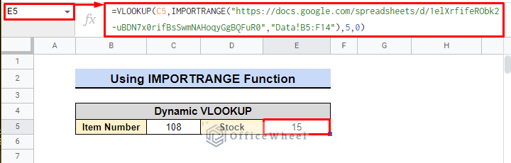
And with that, we have successfully used the VLOOKUP and IMPORTRANGE functions to find the stock count of our toy store products.
Read More: VLOOKUP with IMPORTRANGE Function in Google Sheets
Conclusion
The use of dynamic range in the Google Sheets VLOOKUP function allows for a flexible and efficient way to search for specific data within a large dataset. It eliminates the need for manual updates of ranges, ensuring accuracy and saving time in the process. The dynamic range can be applied in different ways, such as using the INDEX and MATCH functions or the ARRAYFORMULA function, depending on the specific requirement. Check OfficeWheel for more relevant content.
Related Articles
- How to Use Wildcard in Google Sheets (3 Practical Examples)
- Check If Value Exists in Range in Google Sheets (4 Ways)
- [Fixed!] Google Sheets If VLOOKUP Not Found (3 Suitable Solutions)
- How to VLOOKUP for Partial Match in Google Sheets
- VLOOKUP Error in Google Sheets (with Quick Solutions)
- Highlight Cell If Value Exists in Another Column in Google Sheets
- How to Use Nested VLOOKUP in Google Sheets
- Use VLOOKUP to Import from Another Workbook in Google Sheets