Today, we will look at all the ways to return cell reference in Google Sheets. We will utilize some functions that are not often used in day-to-today spreadsheet tasks but can be quite adaptable in many cases.
Let’s get started.
4 Ways to Return Cell Reference in Google Sheets
1. Return Cell Reference Using the ADDRESS Function
For our first example, we will be utilizing the ADDRESS function. This is the simplest way to get the cell reference or address of a cell in Google Sheets.
The ADDRESS Function Syntax
ADDRESS(row, column, [absolute_relative_mode], [use_a1_notation], [sheet])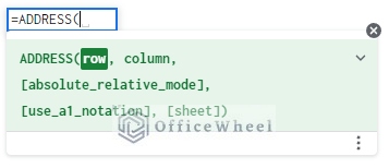
Function Breakdown:
- row: The row number of the cell reference
- column: The column number of the cell reference. Note that this is the number not the letter that is usually associated with columns in spreadsheets.
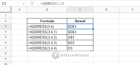
- [absolute_relative_mode]: Optional. This defines whether the returned reference is absolute or not. It has four iterations.
- 1: Both row and column are absolute. ($A$1)
- 2: The row is absolute and the column is relative. (A$1)
- 3: The row is relative and the column is absolute. ($A1)
- 4: Both row and column are relative. (A1)
- [use_a1_notation]: This is Optional and TRUE by default. Determines how the reference is represented
- A1 format (TRUE): Regular cell reference format. (B2, D11, F12)
- R1C1 format (FALSE): Gives the row number and the column number only. (R2C3, R5C2, R10C20)
- [sheet]: Optional. The name of the worksheet. Must be within the same spreadsheet.
Here is a general example of the outcomes:
Basic Example to Return Cell Reference in Google Sheets with the ADDRESS Function
Now let’s consider the following worksheet of random numbers:
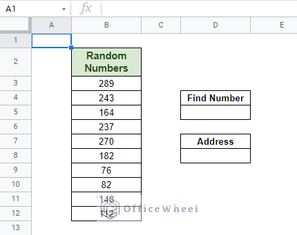
Let’s say we want to find the cell reference or the address of the cell that contains the number 270. To do this, we have to use the combination of ADDRESS and MATCH functions.
=ADDRESS(MATCH($D$5,B3:B12,0),2)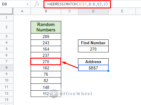
Formula Breakdown:
- The row section is covered by the MATCH function.
- The MATCH function looks up the value given in cell D5 in the given range, column B (B:B), and returns the row number.
- The column section is manually inputted. Since it is column B of our worksheet, the column number is 2.
This concludes the simplest way to return cell reference in Google Sheets. The formula is very versatile and we will be looking at more iterations and uses of it in the following sections of this article.
Read More: Relative Cell Reference in Google Sheets
2. Address of the Minimum/Maximum Value Using ADDRESS
We can improve upon the ADDRESS and MATCH function combination with any other comparative function of Google Sheets to get a variable cell reference.
This time let’s try to find the maximum and minimum integers from the table. Of course, we will be using the MAX and MIN functions for this example.
Cell Reference of the Maximum Value
To find the maximum value in the column, we will apply the MAX function within the MATCH function to get the value we are looking for.
Our formula looks something like this:
=ADDRESS(MATCH(MAX(B3:B12),B:B,0),2)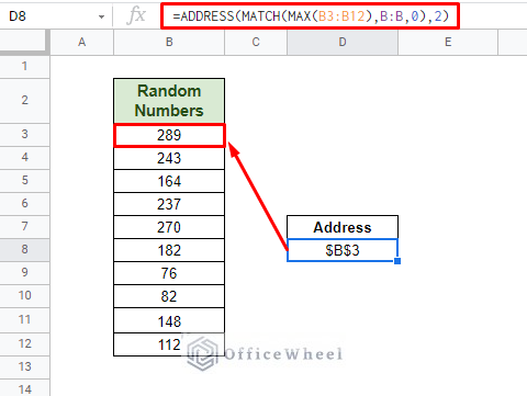
Cell Reference of the Minimum Value
We do the same but with the MIN function this time.
=ADDRESS(MATCH(MIN(B3:B12),B:B,0),2)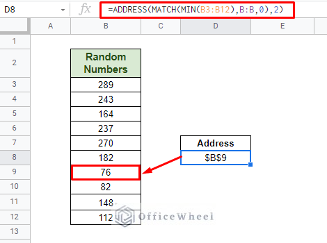
Similar Readings
3. Combining ADDRESS and INDIRECT to Return Cell Reference and Value
We can use the returned cell reference by the ADDRESS function in many ways. One of the ways is to use the output to return a text value. We do this by utilizing the ADDRESS output with the INDIRECT function.
We can see this in the following image:
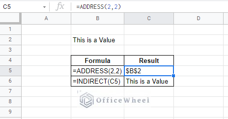
Here, we extract the address of the text “This is a Value” with the ADDRESS function and later use this output in the INDIRECT function to see the cell value as a string.
Another example of the combination of the ADDRESS and the INDIRECT function would be to indirectly reference cells in Google Sheets.
In the following worksheet, we are going to extract a name from the list using the row and column numbers.
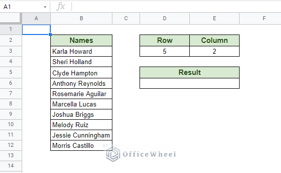
Our formula:
=INDIRECT(ADDRESS(D3,E3))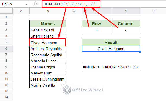
One particular use of this formula would be to find particular values from a table that spans over a large number of rows and columns.
Read More: Indirect Sheet Name in Google Sheets (Easy Steps)
4. Return Cell Reference Using CELL function
This example is to show an alternative to the ADDRESS function that we have been using till now, that is by using the CELL function.
CELL function syntax:
CELL(info_type, reference)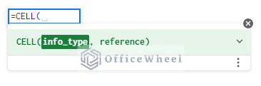
The info_type can be any type of information that we are looking for in a cell. It can be width, row, column, and of course, address of the cell among others. For this particular article, we will focus on the address.
=CELL("address",B4)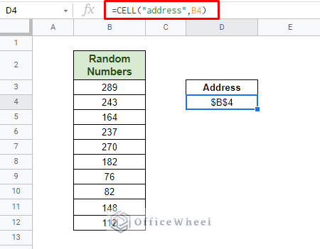
The function in and of itself only returns the absolute reference of the given cell, which is not much. But the CELL function supports expressions as a reference instead of a direct reference that can be useful in formulas.
For example, we can couple CELL with VLOOKUP to find the address of a value from the following table:
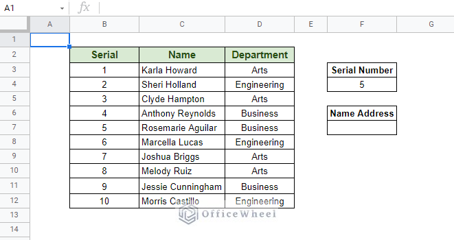
Here, we want to find the cell reference or address of the Name with respect to the given Serial Number.
=CELL("address",VLOOKUP($F$4,B3:D12,2,0))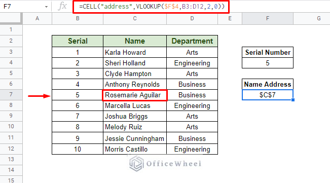
This makes the CELL function more versatile to be used with other functions in Google Sheets, and also removes certain limitations we have seen with the ADDRESS function previously, mainly, working with large tables.
Read More: Google Sheets: Use Cell Value in a Formula (2 Ways)
Final Words
With that, we have covered all the ways we can return cell reference in Google Sheets. Know that the functions we have used are flexible and can be used for more than just returning cell references.
Feel free to leave any queries or advice you might have for us in the comments section below.
Related Articles
- Dynamic Cell Reference in Google Sheets (Easy Examples)
- Reference Another Sheet in Google Sheets (4 Easy Ways)
- Cell Reference From String in Google Sheets
- Reference Another Workbook in Google Sheets (Step-by-Step)
- Pull Data From Another Sheet Based on Criteria in Google Sheets (3 Ways)
- Lock Cell Reference in Google Sheets (3 Ways)