The VLOOKUP function is one of the most useful functions in Google Sheets or Excel. We often use the VLOOKUP function to search any value from a range using a search key and a column index number for the required value. But one of the limitations of using the VLOOKUP function is that the search key must be in the provided range’s first column. In other words, the function searches from left to right. Now, the question arrives: “Can we reverse the VLOOKUP?”. The answer is yes and in this article, I’ll discuss 4 useful ways to do reverse VLOOKUP in Google Sheets.
A Sample of Practice Spreadsheet
You can copy our practice spreadsheets by clicking on the following link. The spreadsheets contain an overview of the datasheet and an outline of the described ways to do reverse VLOOKUP.
4 Useful Ways to Do Reverse VLOOKUP in Google Sheets
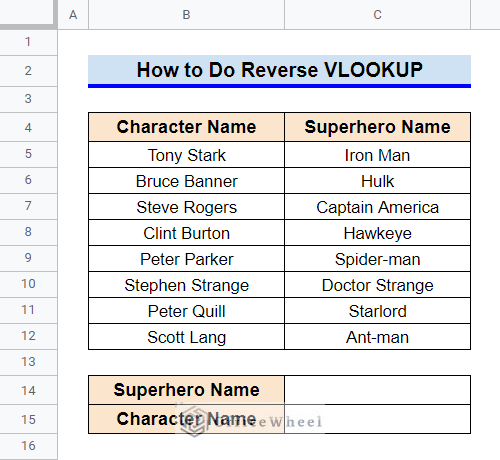
First, let’s get familiar with our dataset. The dataset contains the character names and superhero names of several Marvel Comics characters. The usual VLOOKUP function will find the superhero name based on the character’s name. Here, we will find the character’s name based on the superhero’s name.
1. Using VLOOKUP Function with Virtual Table
One way to reverse VLOOKUP i.e. search from right to left is to create a virtual table where the required columns will be reversed. One point to be noted is that the column that will be reversed doesn’t have to be adjacent.
Steps:
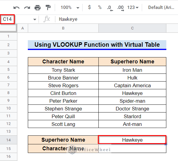
- First, select Cell C14 and then enter any value from the range C5:C12.
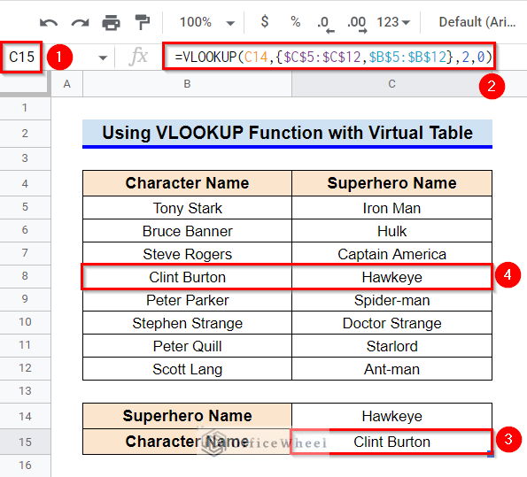
- Afterward, type in the following formula in Cell C15–
=VLOOKUP(C14,{$C$5:$C$12,$B$5:$B$12},2,0)- Here, {$C$5:$C$12,$B$5:$B$12} has created a virtual data table that is the reverse of our dataset.
- Finally, press Enter key to get the required result.
Read More: How to Use VLOOKUP with Drop Down List in Google Sheets
2. Applying XLOOKUP Function
The XLOOKUP function is an alternative to the VLOOKUP function and can help us with reversing the VLOOKUP.
Steps:
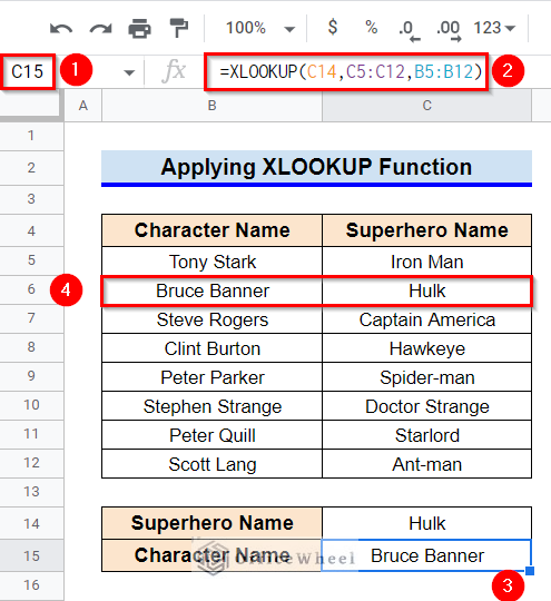
- First, select Cell C15.
- After that, type in the following formula-
=XLOOKUP(C14,C5:C12,B5:B12)- Finally, press Enter key to get the required result.
Read More: How to Use the VLOOKUP Function in Google Sheets
3. Combining INDEX and MATCH Functions
One of the most popular ways to reverse VLOOKUP is to combine INDEX and MATCH functions.
Steps:
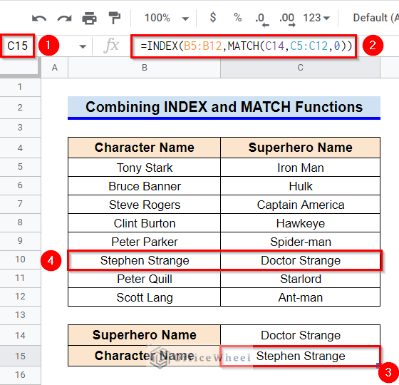
- To start with, select Cell C15.
- After that, type in the following formula-
=INDEX(B5:B12,MATCH(C14,C5:C12,0))- Now, to get the required result, press Enter key.
Formula Breakdown
- MATCH(C14,C5:C12,0)
First, the MATCH function returns the relative position of the search key specified by Cell C14 within the range C5:C12. This relative position works as the row number for the INDEX function.
- INDEX(B5:B12,MATCH(C14,C5:C12,0))
After that, the INDEX function returns the content of the cell where a match is found within range B5:B12.
Read More: Combine VLOOKUP and HLOOKUP Functions in Google Sheets
Similar Readings
- How to Use VLOOKUP with IF Statement in Google Sheets
- VLOOKUP Multiple Columns in Google Sheets (3 Ways)
- How to VLOOKUP with Multiple Criteria in Google Sheets
- Highlight Cell If Value Exists in Another Column in Google Sheets
- How to VLOOKUP Last Match in Google Sheets (5 Simple Ways)
4. Joining INDIRECT and MATCH Functions
Joining INDIRECT and MATCH functions is perhaps the easiest way to reverse VLOOKUP in Google Sheets.
Steps:
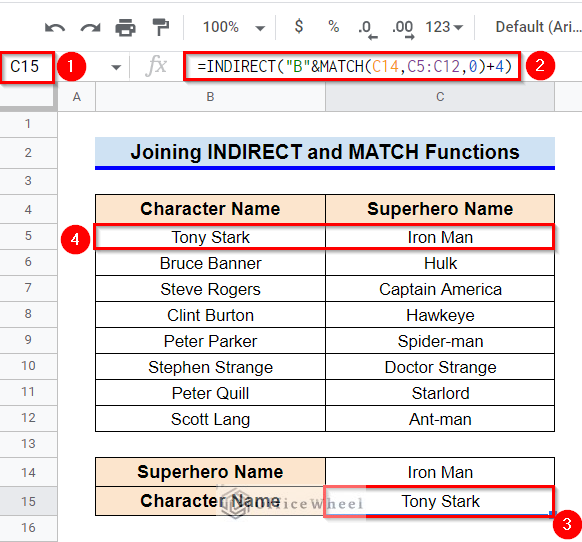
- First, select Cell C15.
- Afterward, type in the following formula:
=INDIRECT("B"&MATCH(C14,C5:C12,0)+4)- Finally, press Enter key to get the required value.
Formula Breakdown
- MATCH(C14,C5:C12,0)
First, the MATCH function returns the relative position of the search key specified by Cell C14 within the range C5:C12.
- “B”&MATCH(C14,C5:C12,0)
Our output will be from Column B. So a string “B” is added for providing cell reference to the INDIRECT function. Therefore, if the MATCH function returns a relative position of 3, we will get a cell reference of B3.
- INDIRECT(“B”&MATCH(C14,C5:C12,0)+4)
The MATCH function returns relative position, whereas the INDIRECT function requires an absolute reference. Therefore we have added 4 to the cell reference to get the actual value.
Read More: How to Use VLOOKUP Function for Exact Match in Google Sheets
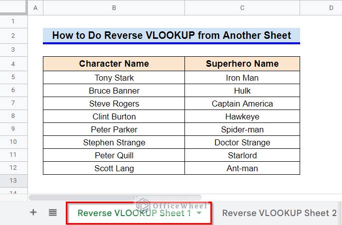
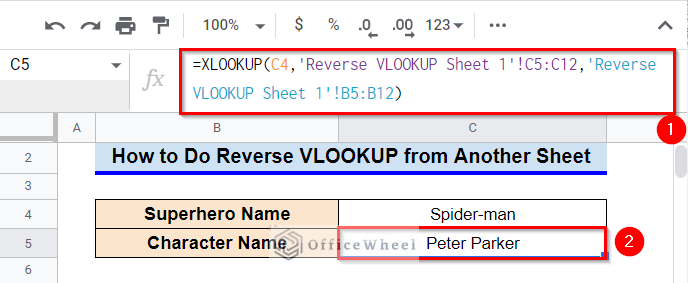
How to Do Reverse VLOOKUP from Another Sheet in Google Sheets
While working on a sheet, we often need to extract data from another sheet. You can use any of the 4 previously discussed methods to reverse VLOOKUP from another sheet. Here, we’ll use the XLOOKUP function.
Steps:
- Here, we will extract data from the worksheet titled “Reverse VLOOKUP Sheet 1”.
- Now, in the workbook titled “Reverse VLOOKUP Sheet 2”, select Cell C5.
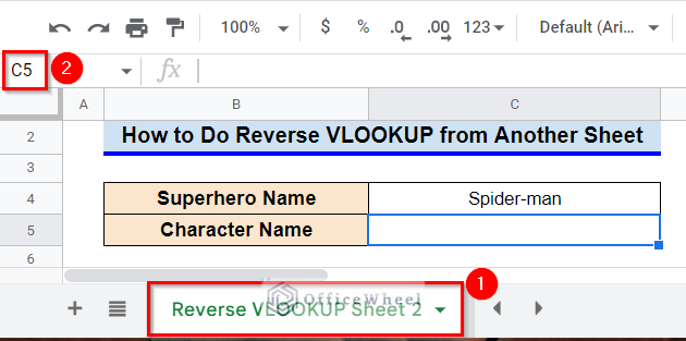
- Now type in the following formula:
=XLOOKUP(C4,'Reverse VLOOKUP Sheet 1'!C5:C12,'Reverse VLOOKUP Sheet 1'!B5:B12)- Press Enter key finally to extract the reverse VLOOKUP.
Read More: How to VLOOKUP from Another Sheet in Google Sheets (2 Ways)
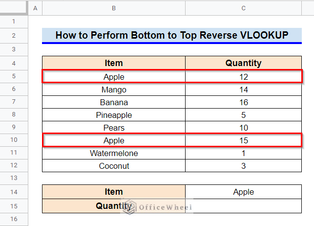
How to Perform Bottom-to-Top Reverse VLOOKUP in Google Sheets
Another limitation of the VLOOKUP function is that it provides search results for the first match only. Therefore, if there are multiple entries for the search key and you require the one from the bottom, you can’t get it using the VLOOKUP function. However, you can combine the INDEX, MAX, FILTER, and ROW functions to perform a bottom-to-top search.
For example, consider the following dataset. It consists of two different rows for the item Apple. We want to extract the bottom one.
Steps:
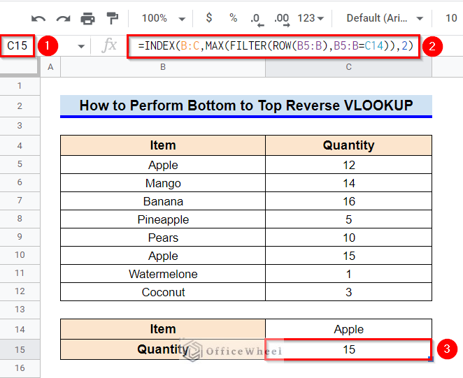
- First, select Cell C15.
- After that, type in the following formula:
=INDEX(B:C,MAX(FILTER(ROW(B5:B),B5:B=C14)),2)- Finally, press Enter key to get the required result.
Formula Breakdown
- ROW(B5:B)
First, the ROW function returns the row number for each cell within range B5:B.
- FILTER(ROW(B5:B),B5:B=C14)
After that, the FILTER function returns the index of the rows where the condition specified by B5:B = C14 is true.
- MAX(FILTER(ROW(B5:B),B5:B=C14)
Next, the MAX function returns the maximum row number (which is in the bottommost) in the dataset returned by the FILTER function.
- INDEX(B:C,MAX(FILTER(ROW(B5:B),B5:B=C14)),2)
Finally, the INDEX function returns the content of the cell from Column C where the criterion matches.
Read More: Create Hyperlink to VLOOKUP Cell in Multiple Rows in Google Sheets
Things to Be Considered
- The MATCH function returns relative cell references whereas the INDIRECT function requires absolute cell references. Therefore, you must add the number of rows prior to the range while joining the MATCH and INDIRECT functions.
Conclusion
This concludes our article to learn how to do reverse VLOOKUP in Google Sheets. I hope the article was sufficient for your requirements. Feel free to leave your thoughts on the article in the comment box. Visit our website OfficeWheel.com for more useful videos.
Related Articles
- How to Use VLOOKUP with Named Range in Google Sheets
- Google Sheets Vlookup Dynamic Range
- How to Use Nested VLOOKUP in Google Sheets
- [Fixed!] Google Sheets If VLOOKUP Not Found (3 Suitable Solutions)
- How to VLOOKUP for Partial Match in Google Sheets
- VLOOKUP Between Two Google Sheets (2 Ideal Examples)
- How to Use IFERROR with VLOOKUP Function in Google Sheets
- Alternative to Use VLOOKUP Function in Google Sheets