Filtering is a primary process that is utilized in most spreadsheets, especially those that contain a large amount of data. While most spreadsheet applications have a built-in filter feature, Google Sheets goes a step further by providing us with the FILTER function.
The function works like a traditional filter with the added bonus of being a function in the application. This means that the conditions are not hard-coded and can be customized to the user’s needs.
What is the FILTER Function of Google Sheets?
The FILTER function of Google Sheets takes a range of data to filter according to the specified condition or conditions.
Syntax for the FILTER function:
FILTER(range, condition1, [condition2, ...])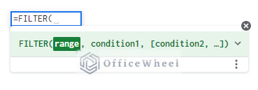
- range: The cell range of the values of the source dataset that will be used to filter.
- condition1: The primary condition to filter the data range by.
- [condition2, …]: (Optional) Secondary condition included beyond the primary condition. More conditions can be added to the FILTER function like this, separated by a comma (,).
The FILTER Function: Basic Use
To show the basic workings of the FILTER function, we have created the following worksheet:
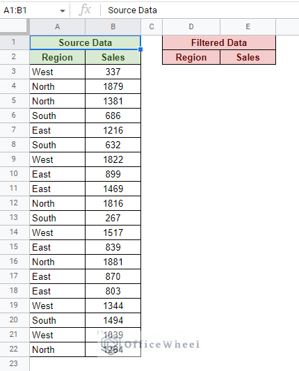
Our objective is to filter all entries that have a Sales value over 1000.
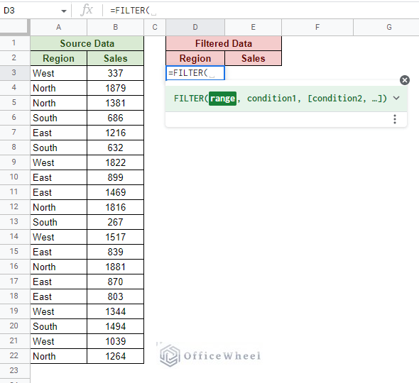
Step 1: Open the FILTER function in the desired cell. Google Sheets helps its users by presenting the syntax of any function automatically.
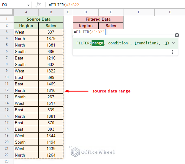
Step 2: Input the data range. This will be all the cells that contain values in the source table.
Step 3: Input the primary filter condition. In this case, it will be greater than 1000. So, we take the range of the column and set the greater than condition.
B3:B22>1000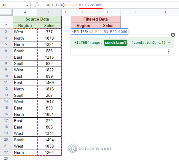
Note: The condition range must be within the data range.
Step 4: Close parentheses and press ENTER. The final formula is:
=FILTER(A3:B22,B3:B22>1000)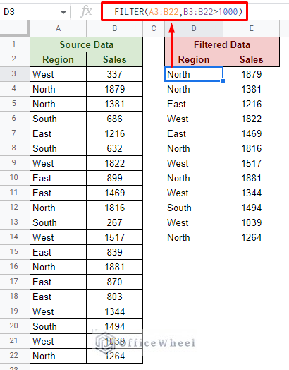
This concludes the basic use of the FILTER function in Google Sheets.
Like most functions in the application, the FILTER function is quite customizable depending on the scenarios it is used in.
The rest of the article focuses on the function’s further use cases and has a look at different common scenarios that users may find themselves in.
Several Use Cases and Scenarios of the FILTER Function in a Google Sheets Worksheet
1. Filter with Multiple Conditions (AND Logical Criteria)
The FILTER function is not confined to working with a single criterion. It can work with multiple different conditions as long as they fall within the data range and the logic of the source data.
In the syntax, we’ve seen that we can add these conditions separated by commas. However, note that adding multiple conditions like this will make them follow the AND logic. This means that the conditions will be dependent on each other.
Let’s see this with an example.
Consider the following worksheet. Here, we want to filter all entries of Bricks that have sold over 1000 units.
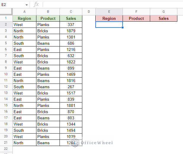
Note that the conditions are Bricks and over 1000 units. These conditions are dependent on each other. So, we can simply use the default way of adding conditions in the FILTER function.
Step 1: Open the FILTER function and select the data range.
Step 2: Input the two conditions separated by a comma.
For Bricks:
B2:B21="Bricks"For Sales over 1000:
C2:C21>1000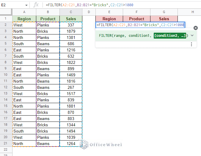
Step 3: Close parentheses and press ENTER to see the results.
=FILTER(A2:C21,B2:B21="Bricks",C2:C21>1000)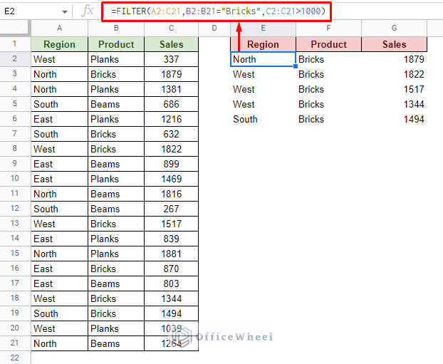
As you can see, both conditions are satisfied.
Read More: Filter with the AND Condition in Google Sheets (An Easy Guide)
2. Filter with Multiple OR Conditions
What if we want to filter for mutually exclusive conditions?
In other words, filtering with OR conditions in Google Sheets.
You’ll be happy to know that it is quite easy to do so. This is with the help of the plus (+) Boolean. And the other difference from the previous multi-condition FILTER formula is that this time we will make use of only one condition field of the function.
So, to filter entries of Bricks or Sales over 1000 units, the condition will be:
(B2:B21="Bricks")+(C2:C21>1000)Note: Each of the conditions is enclosed within parenthesis. This is to represent them as individual conditions that are connected with an OR condition (+).
Applying this condition to the FILTER function:
=FILTER(A2:C21,(B2:B21="Bricks")+(C2:C21>1000))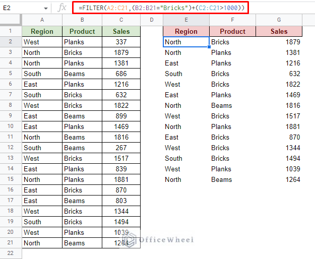
It is important to also note that in the previous two examples we have shown how to work with two conditions. But that is not the limit.
You can add as many conditions as you require.
- For the AND multiple criteria, separate the conditions with a comma (,).
- For the OR multiple criteria, separate the conditions with a plus (+). Again, this will only cover a single condition field of the FILTER function
Read More: Google Sheets: Filter for Multiple Criteria with Formula (2 Easy Ways)
3. Referencing Conditions or Criteria from a Different Cell
One of the biggest advantages of using the FILTER function over the default filter of Google Sheets is that we can use a cell reference as a condition or criteria.
Consider the first dataset we have shown in this article. Let’s say we want to filter by the Region values. Normally, we’d have had to input the text North, South, East or West within the condition field of the formula.
=FILTER(A3:B22,A3:A22="North")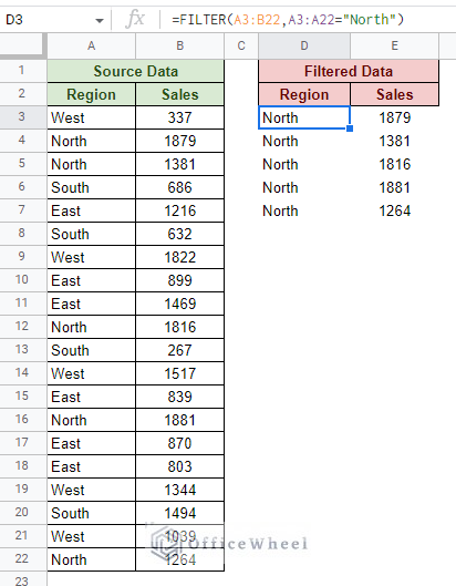
But let’s instead try to reference this value from a different cell. All we have to do is apply a cell reference in the place of “North” and make sure that this reference is locked in absolutes ($) so that the reference does not move around in the formula.
=FILTER(A3:B22,A3:A22=$G$2)Tip: To cycle through different cell reference locking conditions, press the F4 key of the keyboard when the text cursor is over the cell reference.
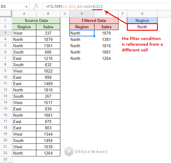
As you can see, the formula correctly recognizes the text that is in a different cell using cell reference.
Drop-down Menu Example
Let’s make the method more dynamic by adding a drop-down menu of possible conditions. Skip them if you already know how.
For adding a drop-down menu, for Regions in this example, follow these steps:
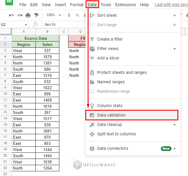
Step 1: Navigate to the Data tab and select the Data validation option.
Step 2: In the Data validation window, apply the following conditions highlighted in the image. Namely the Criteria and “Reject input” options.
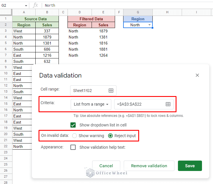
Step 3: Click Save to apply the drop-down menu for Region.
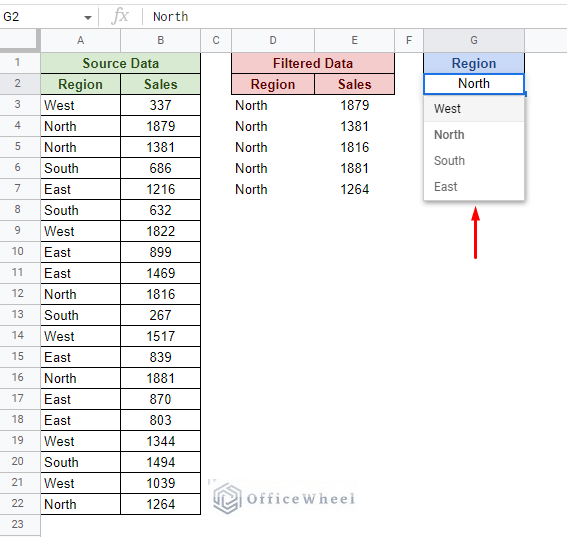
Now, if we change this value, the FILTER formula results will change accordingly:
Read More: How to Use Data Validation and Filter in Google Sheets (4 Ways)
4. Filter the Top N-Number of Values in Google Sheets
A common filter condition is to find the top n-number of values of a dataset. Thanks to the FILTER function, the method is no longer complicated as it might have been with the default filter of Google Sheets.
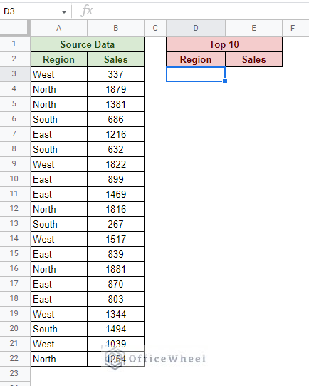
We will use the following dataset to find the top 10 Sales value:
The customization we need to bring is in the condition field. To filter the Top 10 values from a dataset, we must utilize the LARGE function in the condition field of the FILTER function.
LARGE(data, n)Where:
- “data” will be the range of values in the specified column. In this case, the Sales column.
- “n” will act as the number of values that we want to filter. Since we want the top 10, the value of “n” will be 10.
So, the condition will be something like this:
(B3:B22>=LARGE(B3:B22,10))Making the final formula to be:
=FILTER(A3:B22,(B3:B22>=LARGE(B3:B22,10)))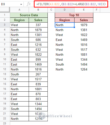
If you want a different number of the top values, e.g., top 3, top 5, and so on, simply change the value of “n” in the LARGE function.
Extra: For the Bottom 10 Values
Similarly, we can also filter the bottom 10 values from the dataset. We only need to bring two changes:
- Set the logical calculation to less than or equal to (<=).
- Use the SMALL function instead.
The formula:
=FILTER(A3:B22,(B3:B22<=SMALL(B3:B22,10)))
Read More: Google Sheets: Filter Data if it Contains Value (A Comprehensive Guide)
Similar Readings
- How to Filter with QUERY for Multiple Criteria in Google Sheets (An Easy Guide)
- How to Filter Based on a Cell Value in Google Sheets (2 Easy ways)
- Filter Data Using Filter Views in Google Sheets (An Easy Guide)
- How to Delete Filter Views in Google Sheets (An Easy Guide)
- Google Sheets: The VALUE Function (An Easy Guide)
5. Sort Filtered Data in the Same FILTER Formula
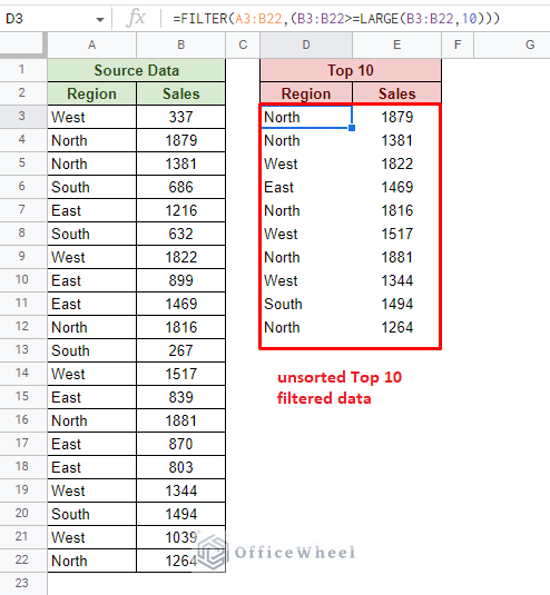
Let’s continue from where we left off with filtering the top 10 values in Google Sheets. Recall that the results that were produced were not sorted. This begs the question: How do we sort filtered data in Google Sheets?
We once again take advantage of the fact that FILTER is a function and can be combined with others quite easily.
The other function in question this time is obviously the SORT function.
The SORT function syntax:
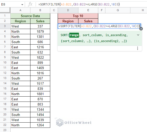
SORT(range, sort_column, is_ascending, [sort_column2, is_ascending2, ...])Let’s go through the process step by step:
Step 1: Open the SORT function first. From the function’s syntax, we can see the range field. This will be covered by the FILTER formula.
For this example, it is the Top 10 FILTER formula:
Step 2: Move to the next field, the sort_column. This represents the column index that the SORT function will sort the values by. In this case, it is column 2 (Sales).
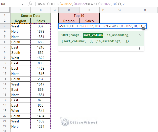
Step 3: Set the is_ascending field to FALSE since we want the results to show the highest values first.
Step 4: Close parentheses and press ENTER to see the results.
=SORT(FILTER(A3:B22,(B3:B22>=LARGE(B3:B22,10))),2,FALSE)Read More: How to Filter by Condition Using a Custom Formula in Google Sheets (3 Easy Examples)
6. Filter for the “Does not contain value” Condition in Google Sheets
This condition is usually used alongside filters to match strings or partial text in Google Sheets.
To that end, this section will focus on these two conditions for the FILTER function:
- A matching text. Partial or otherwise.
- A Boolean criterion for the “does not contain value” condition.
Both of these conditions can be applied with the regular expression function, REGEXMATCH.
For this example, let’s try to filter all Regions except East.
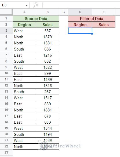
Step 1: Open the FILTER function and input the data range.
Step 2: Input the condition. To find the text match, the formula will be:
REGEXMATCH(A3:A22,"East")To apply the “does not contain value” criteria to this we must add a Boolean:
REGEXMATCH(A3:A22,"East")=FALSE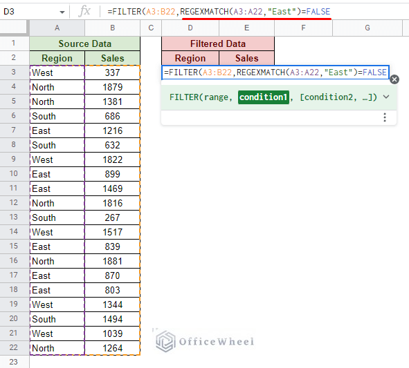
Step 3: Close parentheses and press ENTER.
=FILTER(A3:B22,REGEXMATCH(A3:A22,"East")=FALSE)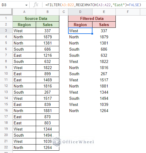
As you can see, all entries except those containing the “East” Region data have been presented.
Read More: Filter Entries if it Does Not Contain Value in Google Sheets (2 Easy Ways)
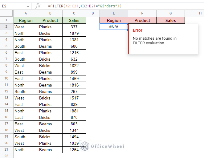
7. What happens when there are no matches for the FILTER function in Google Sheets?
For any of the previous scenarios, there may be a dataset that does not satisfy any condition. And thus, it will result in an error:
There is no solution to this beyond doing some error handling with the IFERROR function.
=IFERROR(FILTER(A2:C21,(B2:B21="Girders")),"")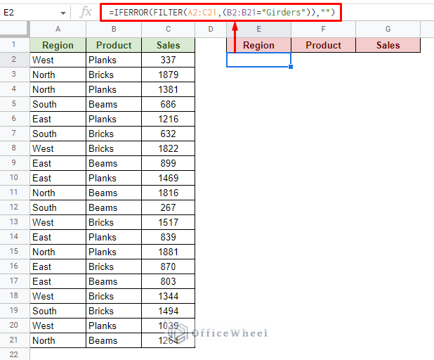
Mismatched Rows and Columns for FILTER conditions
Speaking of errors, the FILTER function cannot take different ranges of rows and columns as a condition. This will result in an error.
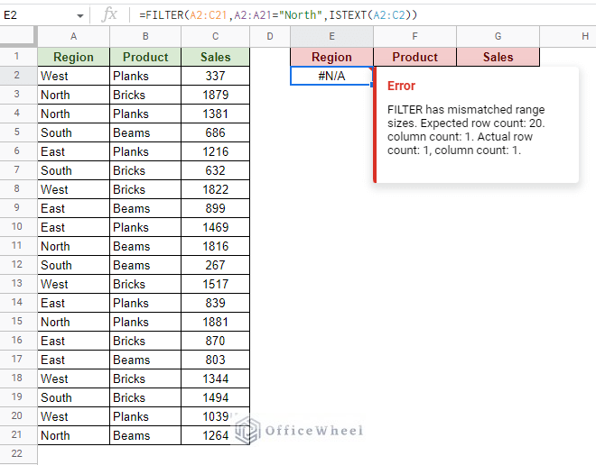
Here you can see that both conditions have a different range of data that they work with. This kind of mismatched range cannot be computed by the FILTER function.
Read More: How to Filter By Rows in Google Sheets (An Easy Guide)
Final Words
That concludes our simple guide on how to use the FILTER function in Google Sheets. Not only is the function able to filter data according to the specific conditions of the user, but it also comes with all the advantages a function has in Google Sheets. Mainly customizability.
We hope that this article was able to give you a better understanding of the different use cases of the FILTER function and that you will now be able to utilize it in your spreadsheets.
Feel free to leave any queries or advice you might have for us in the comments section below.
Related Articles
- How to Find and Replace Blank Cells in Google Sheets
- How to Use Wildcard in Google Sheets (3 Practical Examples)
- Applying Filter with REGEXMATCH Function in Google Sheets (Easy Examples)
- Filter Values that Contains Multiple Text Criteria in Google Sheets (2 Easy Ways)
- Google Sheets: Filter Data that Contains Text (3 Easy Ways)
- How to Autofill Formula in Google Sheets (3 Easy Ways)