In Google Sheets, with the help of an asterisk wildcard (*) in the VLOOKUP function, you can look up values that have a partial match with certain text instead of the exact match of the values. In this article, we will learn about VLOOKUP partial match in Google Sheets.
A Sample of Practice Spreadsheet
You can download spreadsheets from here and practice.
3 Ideal Examples to VLOOKUP for Partial Match in Google Sheets
The asterisk wildcard represents a number of characters. For example, the string ‘Wh’ can represent What, When, Who, Where, etc. So, if you want to look up any value that may not exactly match your dataset, you can put this wildcard in the VLOOKUP function and get the desired result.
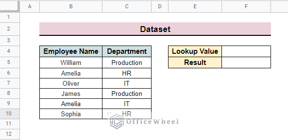
You can use this asterisk wildcard (*) to look up a partial match from the beginning, end middle of the test. Here, we develop a dataset containing two columns namely: Employee Name, and Department. We also add Lookup Value and Result in rows to apply the function in the dataset.
In the VLOOKUP function, the use of wildcards depends on the partial text type.
1. Match Partial Text
The most common type of looking up partial values is text values. These match conditions can be found in three locations of a text: beginning, middle, or end.
I. Beginning of Text
To look up the value that has a partial match with the beginning of the exact text in the dataset,
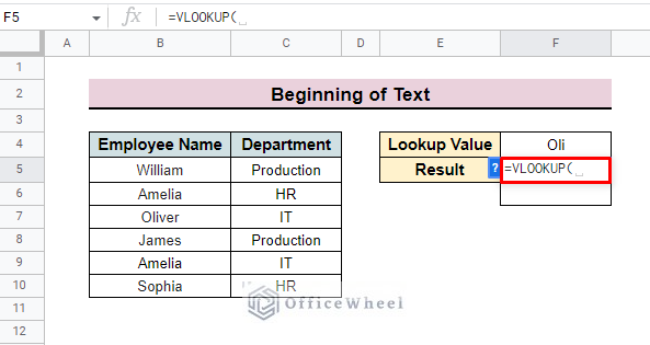
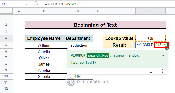
- First insert the partial value in the Lookup Value cell. Here we add ‘Oli’ as a partial match.
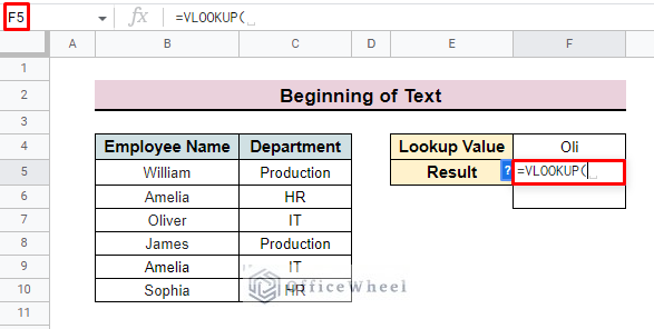
- Then apply the VLOOKUP function in the Result cell F5.
- Now, input the partial match value as search key.
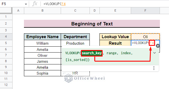
- After that add ‘&’ and an asterisk (*). The * wildcard represents any value after the data in cell F4.
- Whereas the & symbol joins the cell reference and the wildcard into one statement.
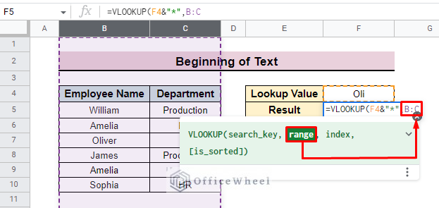
- Then insert the range in the function. Here, we add the entire dataset as range B:C in the function.
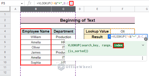
- Add the index value 1. Here, 1 represents the column number of the data table.
- Set the is_sorted parameter to FALSE to extract the exact value.
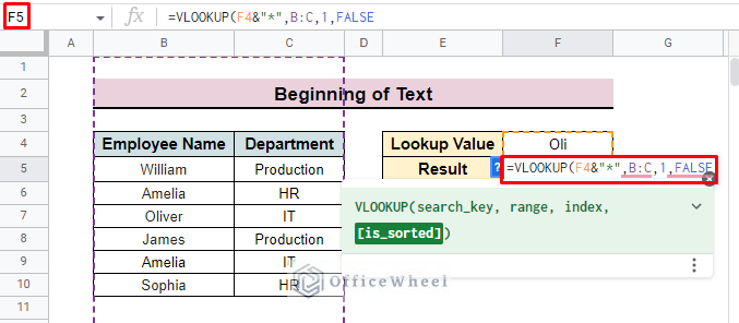
- Finally, press ENTER to get the desired value in the selected cell,
=VLOOKUP(F4&”*”,B:C,1,FALSE)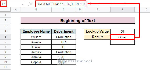
- You can apply the same function to the second column of the dataset. In that case, you just change the column number in the function. The rest of the function will be the same.
=VLOOKUP(F4&”*”,B:C,2,FALSE)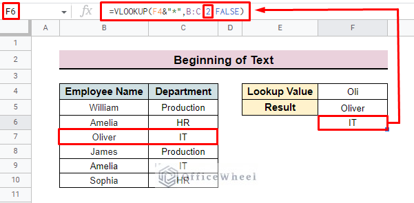
Read More: How to Use Wildcard in Google Sheets (3 Practical Examples)
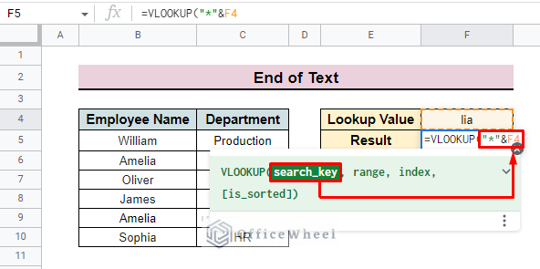
II. End of Text
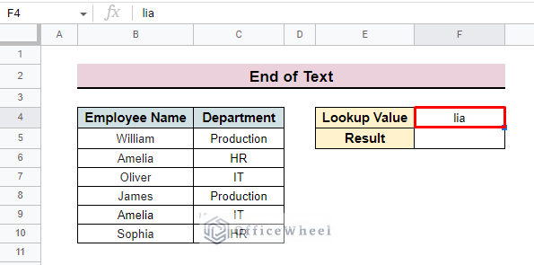
If the partial value represents the end of the text, then there is a slight difference in function. In that case,
- First of all, input the partial value that you have in the Lookup Value cell.
- Then insert the VLOOKUP function in cell F6. In the function first, add the “*” character.
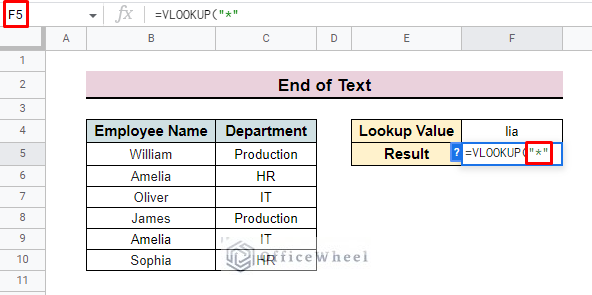
- After the wildcard character, use the ‘&’ symbol as a connector and add the F4 cell as the search key of the function.
- After that insert range, index, and is_sorted as like we show in the previous one.
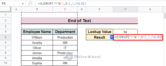
- In the end, press ENTER to input the outcome in your selected cell.
=VLOOKUP(“*”&F4,B:C,1,FALSE)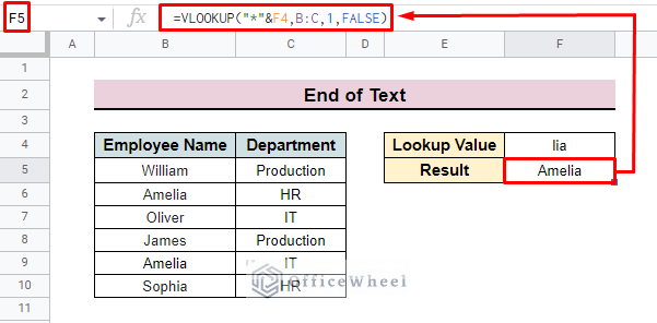
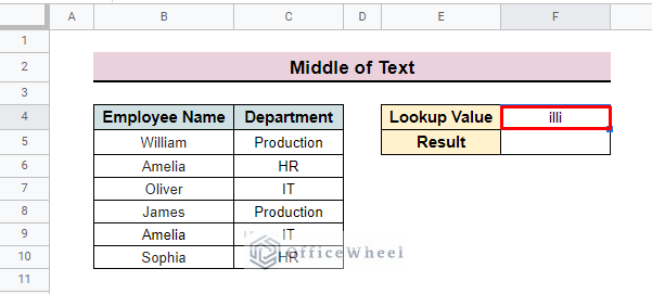
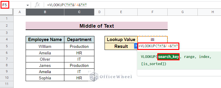
III. Middle of Text
If the partial match value contains the middle portion of the exact text, then the VLOOKUP function will be a little bit complex. To look up the middle of the text,
- At first, add the partial match in the Lookup Value cell. Here, we add ‘illi’ as our lookup value. It contains the middle portion of an employee’s name.
- Apply the VLOOKUP function then adds “*” at the beginning. As the beginning and end text is unknown, so insert the “*” wildcard character before and after the search key. Connect the whole statement with the ‘&’ symbol. Here, we add the F4 cell as the search key.
- After that input the rest of the function as per the previous instruction.
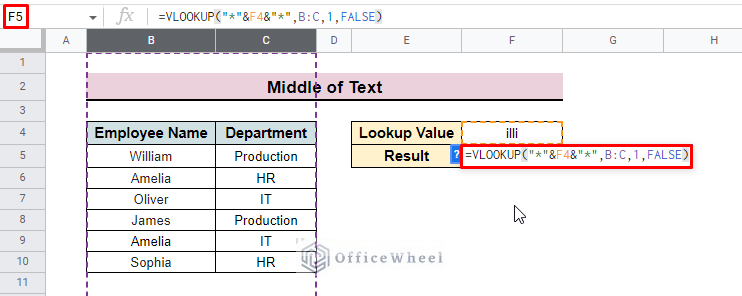
- Finally, apply the Final formula in cell F5 and find the desired result. Here we find ‘William‘ as final outcome.
=VLOOKUP(“*”&F4&"*",B:C,1,FALSE)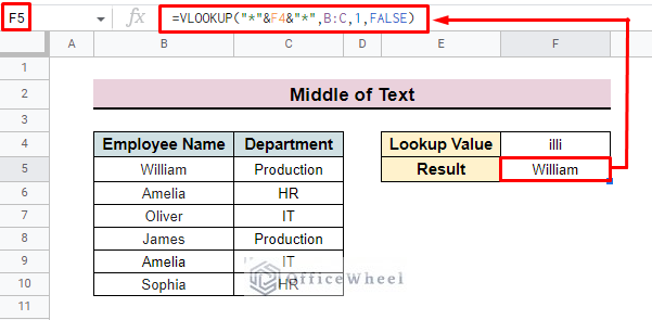
Similar Reading:
- Create Hyperlink to VLOOKUP Cell in Multiple Rows in Google Sheets
- How to Use IFERROR with VLOOKUP Function in Google Sheets
- Alternative to Use VLOOKUP Function in Google Sheets
- How to Use VLOOKUP for Conditional Formatting in Google Sheets
- VLOOKUP Multiple Columns in Google Sheets (3 Ways)
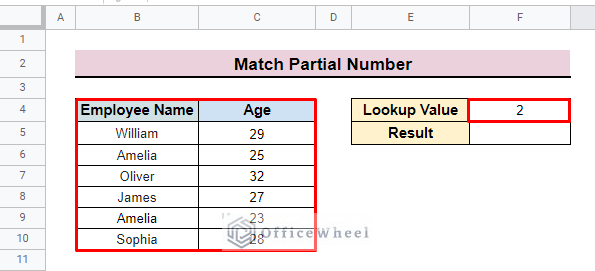
2. Match Partial Numbers
You can also apply the partial match value to look up Numeric data as well as dates from your dataset. Generally, the VLOOKUP search key does not support numeric value, but by modifying the formula we can extract both the number and date from the dataset.
For looking up numbers from the dataset through partial numbers with the VLOOKUP function, we have to apply the ARRAYFORMULA function. To do so,
- First, develop a dataset containing number values. Here, our dataset represents Employee Name and Age columns. Besides, we input 2 as the Lookup Value.
- Then in cell F5 apply the formula.
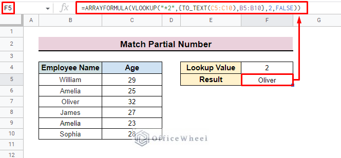
=ARRAYFORMULA(VLOOKUP(“*2”,{TO_TEXT(C5:C10),B5:B10},1,FALSE))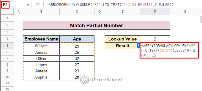
Formula Breakdown
- TO_TEXT(C5:C10): Here, C5:C10 is the age range which represents in numeric form. The TO_TEXT function converts the numeric range to the text range.
- B5:B10: This is the text range that represents the Employee Name.
- “*2”: It represents the search key for the VLOOKUP function.
- 2: This is the column number and FALSE is set as is_sorted to extract the exact value.
- VLOOKUP(….): Here, the function lookup for a numeric value that ends with 2 where the TO_TEXT function helps to convert the numeric value to the text.
- ARRAYFORMULA(…..): Here, the ARRAYFORMULA function is used to support the non-array TO_TEXT function.
- Press ENTER to apply the formula in the F5 cell and find the full numeric value that exist in the main dataset.
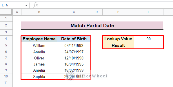
3. Match Partial Dates
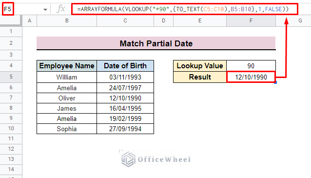
You can use the same formula to look up dates in the dataset. Here, we use a dataset representing Employee Name and Date of Birth. We look up values ending with 90.
- Like we did before, we will apply the following formula in cell F5.
=ARRAYFORMULA(VLOOKUP(“*90”,{TO_TEXT(C5:C10),B5:B10},1,FALSE))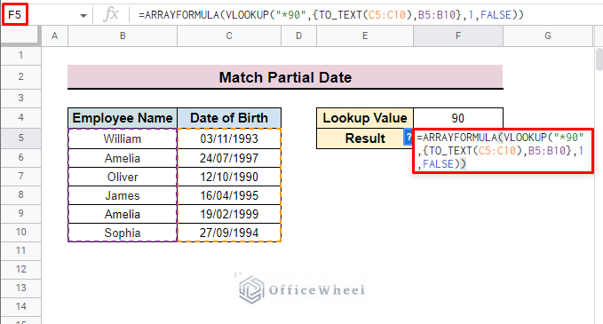
- Click ENTER to insert the function and you will find the full date in your selected cell.
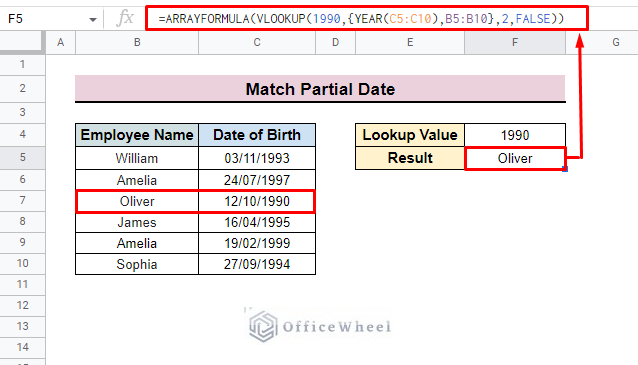
- If you want to look up other columns with the help of the year value, then you can apply this formula as well.
=ARRAYFORMULA(VLOOKUP(1990,{YEAR(C5:C10),B5:B10},2,FALSE))- After applying the function, you will find the respective employee name ‘Oliver’ whose date of birth is ‘1990’.
Formula Breakdown
- YEAR(C5:C10): Here, C5:C10 is the age range which represents in numeric form. The YEAR function converts the numeric year to text.
- B5:B10: It is the text range that represents the Employee Name.
- “*2”: This is the search key for the VLOOKUP function.
- 1: It is the column number and FALSE is set as is_sorted to extract the exact value.
- VLOOKUP(…): Here, the function looks for a numeric value that ends with 2 whereas the YEAR function helps to convert the numeric value to the text.
- ARRAYFORMULA(….): Here, the ARRAYFORMULA function is used to support the non-array YEAR function.
Read More: How to VLOOKUP All Matches in Google Sheets (2 Approaches)
Conclusion
After completing the article, we will hope that you can solve any type of problems related to VLOOKUP partial match in Google Sheets. For any queries feel free to comment and for deeper knowledge, you can also visit the OfficeWheel website.
Related Articles
- Google Sheets Vlookup Dynamic Range
- How to Use VLOOKUP with Named Range in Google Sheets
- How to Use Nested VLOOKUP in Google Sheets
- How to Check If Value Exists in Range in Google Sheets (4 Ways)
- [Fixed!] Google Sheets If VLOOKUP Not Found (3 Suitable Solutions)
- Combine VLOOKUP and HLOOKUP Functions in Google Sheets
- How to Use VLOOKUP with Drop Down List in Google Sheets
- How to Use VLOOKUP to Import from Another Workbook in Google Sheets