Most of the functions in Google Sheets are designed for vertically arranged data. But horizontally arranged data needs horizontal data retrieving. In such arrangements, the HLOOKUP function is useful to retrieve data from a column using the value of the top row as a search key. This article discusses how to perform a horizontal lookup using HLOOKUP and other functions to return an entire column in Google Sheets.
A Sample of Practice Spreadsheet
You can download the spreadsheets from the link below. After downloading you can practice on your own as we demonstrate here.
Introduction to HLOOKUP Function in Google Sheets
Objective
The objective of the HLOOKUP function in Google Sheets is to horizontally lookup and extract data from specified rows.
Syntax
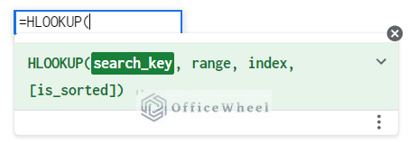
Inputs
- search_key: The value to look for.
- range: The range where to look up the value.
- index: The row number of the value to return.
- [is_sorted]: Takes boolean values depending on the exact or approximate match. For an exact match, it is FALSE, and TRUE for an approximate match.
Output
- Returns specified rows that matched the search key.
3 Simple Ways of Google Sheets HLOOKUP to Return Column
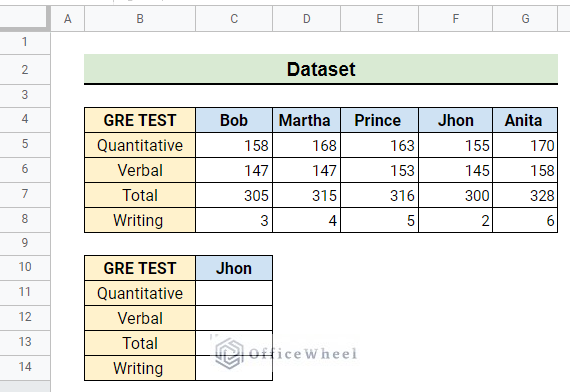
In our dataset, the results of test takers at different sections of an exam are given. We want to horizontally lookup and return the entire column of a test taker’s result using their name as the search key.
1. Using HLOOKUP Function
The HLOOKUP function searches the search key across the first row. We can easily extract specified cells or an entire column of the search key using this function.
Steps:
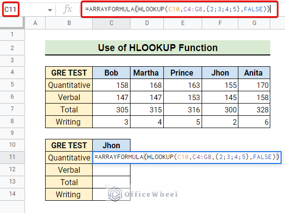
- First, select the cell where you want to return the matched column using the HLOOKUP function. Here, we select cell C11.
=ARRAYFORMULA(HLOOKUP(C10,C4:G8,{2;3;4;5},FALSE))
- Then we insert the above formula in the formula bar.
Formula Breakdown
- C10 is the search key that the HLOOKUP function is looking for.
- C4:G8 is the search range where the HLOOKUP is searching the search key.
- {2;3;4;5} is the index of the search range that will return if the HLOOKUP function finds a match.
- FALSE is used for the HLOOKUP function to find an exact match.
- Finally, ARRAYFORMULA returns an array of specified indexes from the matched column.
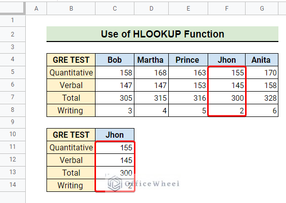
- After inserting the formula we have to press enter. This gives us the entire column that matched the search key as follows.
Read More: Combine VLOOKUP and HLOOKUP Functions in Google Sheets
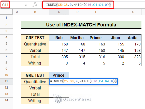
2. Applying INDEX-MATCH Formula
The combination of INDEX and MATCH functions can perform the above task as well. Initially, the MATCH function returns the column index. Then, the INDEX function returns the entire column.
Steps:
- At first, we select cell C11 in which we want to return the matched column as earlier.
=INDEX(C5:G8,0,MATCH(C10,C4:G4,0))
- Then we write down the above formula in the formula bar.
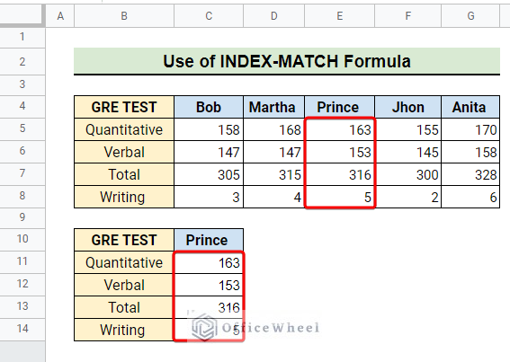
Formula Breakdown
- C10 is the search key for the MATCH function.
- C4:G8 is the search range where the MATCH function is searching the search key.
- 0 means the function will go for an exact match.
- MATCH(C10,C4:G4,0) returns the index of the search key if matched. This passes as the last argument of the INDEX function.
- Finally, using the return of the MATCH function as column index, INDEX(C5:G8,0,MATCH(C10,C4:G4,0)) returns the column within the range of C5:G8.
- Then we press enter and get the entire column that matched.
Read More: Using INDEX MATCH in Google Sheets – A Deep Dive
3. Utilizing XLOOKUP Function
The XLOOKUP function can perfectly replace the HLOOKUP function in the case of horizontal lookup. For that, we have to select a row as the lookup range of the XLOOKUP function.
Steps:
- First, we select cell C11 for horizontal lookup as earlier.
=XLOOKUP(C10,C4:G4,C5:G8)
- Then we insert the above formula in the formula bar.
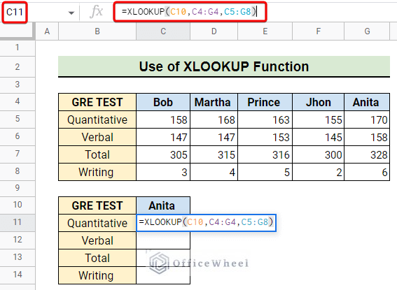
Here, XLOOKUP horizontally lookup the search key C10 within the range C5:G8.
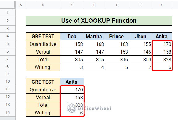
- Finally, pressing enter gives us the following desired output.
Things to Remember
- Try to search for an exact match using the HLOOKUP function. An approximate search may not result in the desired output.
- Make sure the lookup row of the XLOOKUP function is a single row.
Conclusion
In conclusion, I hope from now on you can use the above functions for the HLOOKUP function to return column in Google Sheets on your own. Further, If you have any questions regarding this article feel free to comment below and I will try to reach out to you soon. Visit our website OfficeWheel for the most useful articles.
Related Articles
- How to HLOOKUP for Multiple Criteria in Google Sheets (2 Ways)
- How to Search for Text in Range in Google Sheets (4 Simple Ways)
- [Fixed!] INDEX MATCH Is Not Working in Google Sheets (5 Fixes)
- Google Sheets Conditional Formatting with INDEX-MATCH
- Use of Google Sheets INDEX MATCH in Multiple Columns
- Alternative to Use VLOOKUP Function in Google Sheets
- How to Create Conditional Drop Down List in Google Sheets
- Find All Cells With Value in Google Sheets (An Easy Guide)