Today we will look at how we can use cell value in a formula in Google Sheets. The general idea revolves around cell references, but we will go the extra mile to discuss all types of it.
Let’s get started.
Using Cell Value in a Formula in Google Sheets
1. Using Regular Reference for Cell Value in a Formula in Google Sheets
The most common way to use a cell’s value in a formula in Google Sheets is through cell references. Any spreadsheet user worth their salt knows what cell references are. But what can be slightly complex to understand are the different types of cell references that are available and how to efficiently use them.
Here we have a simple dataset of random integers that we are going to average in a different cell.
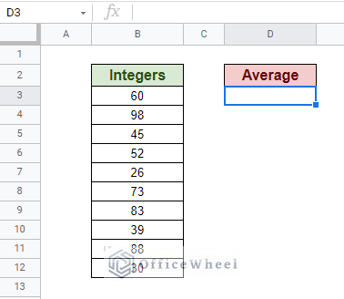
We will be using the AVERAGE function to create a formula by referencing the cell values in the integer column.
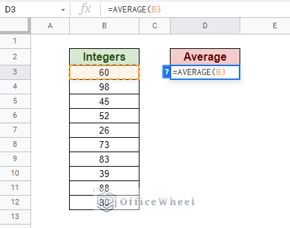
The AVERAGE function takes a range of values, and our integer range starts from cell B3, this is the cell reference. So we use that in the formula.
The final cell of the range of integers is cell B12. The colon (:) in between the cell references denotes the range B3 to B12. Our formula:
=AVERAGE(B3:B12)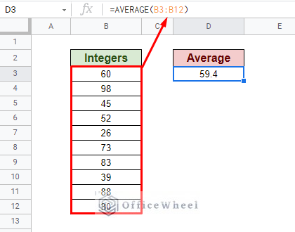
In layman’s terms: We have averaged the cell values from B3 to B12 using the AVERAGE formula.
This is something most spreadsheet users already know. So, what happens when we have multiple sources of values? Or when we want to apply our formula to entire rows and columns?
In such cases, we need to lock our cell references to make these complex conditions work.
Absolute Cell Reference
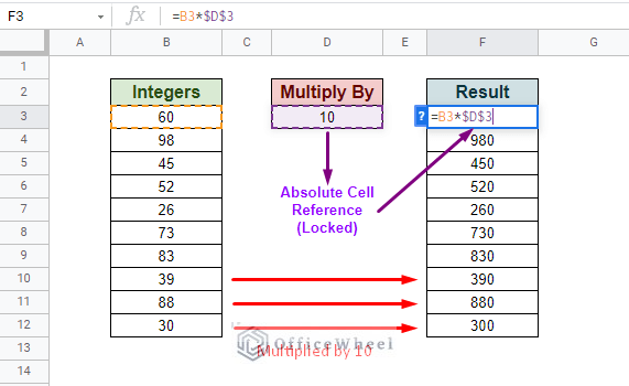
Now, if we want to multiply our integers by, let’s say, 10, we have to make sure that all the results are visible and all the integers are multiplied by the value in cell D3.
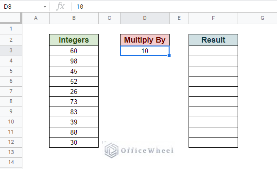
The formula:
=B3*$D$3The value of cell D3 is locked with absolutes ($) so that as we move the formula down the Result column with the fill handle, the values of the Integer column change but the 10 in D3 doesn’t.
Mixed Cell Reference
All cells have a Column Reference (letters: A, B, C…) and a Row Reference (numbers: 1, 2, 3…), and we can lock them separately. Doing so, we get something called Mixed Cell Reference.
For this example, we have added a few more columns of data.
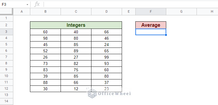
We will use the same AVERAGE function, but for the first example, we will average by row. And to show mixed cell reference, we will lock the column reference only.
=AVERAGE($B3:$D3)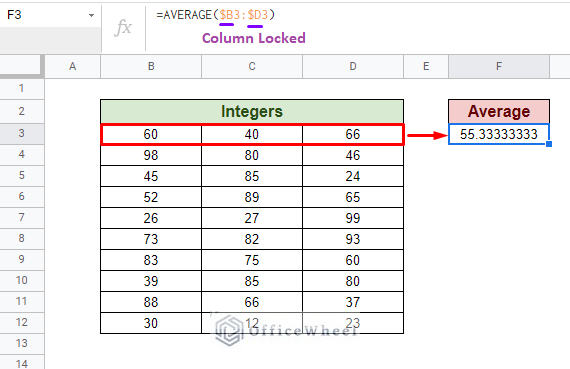
So if we use the fill handle horizontally, the column value won’t increase keeping the formula as it is. If we use the fill handle vertically, the column value again won’t change but the row values will.
Now, the opposite effect happens when we lock the row number of our cell reference. Let’s say we want to find the average by columns this time. Our formula:
=AVERAGE(B$3:B$12)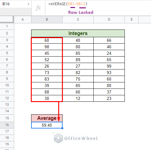
Now, if we use the fill handle horizontally, the column number is free to change. But if we use the fill handle vertically, the row number remains unchanged.
For an in-depth breakdown of everything we have discussed so far, follow our Lock Cell Reference in Google Sheets article.
The idea is when inputting or highlighting a cell reference, pressing the F4 key will transform the current cell reference into different types.

Read More: Find Cell Reference in Google Sheets (2 Ways)
2. Dynamically Reference Cell Value in a Formula in Google Sheets (INDIRECT Function)
The word dynamic implies that this will be somewhat of an advanced method. As such, we will be using one of Google Sheets’ heavy-hitting functions, the INDIRECT function to use cell value in a formula. As a function, INDIRECT has amazing uses but it is also very easy to get wrong.
It is better shown with an example. The core of using INDIRECT is when we are using it to reference a cell from another cell (dynamically).
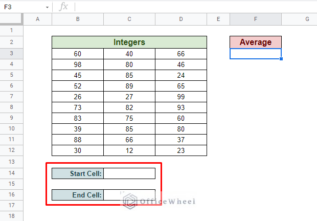
Here, we have made some modifications to our previous dataset. We have added the Start Cell and End Cell targets. We will use these targets to dynamically reference the start and the end of the range for our average. Meaning, the values of these cells are indirectly referenced.
Now, if we want to find the average value from cell B3 to C8 from the Integers table, we simply designate the Start Cell as B3 and End Cell as C8 for our formula:
=AVERAGE(INDIRECT(C14&":"&C16))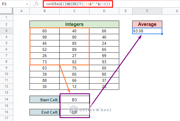
Not only for the AVERAGE function but INDIRECT can also be used to passively reference any cell for any function, for both the same or different worksheets.
To see these examples of the in-depth usage of INDIRECT, please see our Dynamic Cell Reference in Google Sheets article.
Read More: Relative Cell Reference in Google Sheets
Final Words
That concludes all the general ways we can use cell value in a formula in Google Sheets. Note that we go much more in-depth on other articles dedicated to each method mentioned here. You can find the links to those articles at the end of each method.
Feel free to leave any queries or advice you might have for us in the comments section.
Related Articles
- Reference Another Workbook in Google Sheets (Step-by-Step)
- Pull Data From Another Sheet Based on Criteria in Google Sheets (3 Ways)
- Reference Another Sheet in Google Sheets (4 Easy Ways)
- Cell Reference From String in Google Sheets
- Variable Cell Reference in Google Sheets (3 Examples)
- Reference Another Tab in Google Sheets (2 Examples)