How to Use VLOOKUP to Import from Another Workbook in Google Sheets

When working with a large volume of data it can be tiring and time-consuming to go back and forth to look for specific data. In that case, Google Sheets provides VLOOKUP function that saves you time and trouble by looking up specific data for you. In this article, we will try to learn how to VLOOKUP from another workbook in Google Sheets easily and effectively in a simple way.

Table of Contents hide

What Is the VLOOKUP Function?

Step by Step Process of Using VLOOKUP to Import Data from Another Workbook in Google Sheets

Step 1: Preparing Datasets

Step 2: Getting Started with VLOOKUP

Step 3: Imposing IMPORTRANGE

Step 4: Importing Data Using IMPORTRANGE

Step 5: Finalizing VLOOKUP

Step 6: Final Look

Conclusion

What Is the VLOOKUP Function?

VLOOKUP means vertical lookup in short. VLOOKUP lets you look for a particular value down the first column in a range of cells. This is what the formula looks like in Google Sheets:

=VLOOKUP(search_key, range, index, [is_sorted])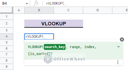

search_key: It indicates the value to look for in the specified range.
range: range denotes the table to consider for the look up.
index: index indicates column number in the range table. The index must be a positive integer.
is_sorted: Optional input. Choose an option between the following two:
FALSE means Exact match. This is recommended.
TRUE means Approximate match. This is the default if is_sorted is unspecified.

VLOOKUP searches the leftmost column in the range and returns a value from the matching row in the cell identified by index.

Step by Step Process of Using VLOOKUP to Import Data from Another Workbook in Google Sheets

So, what do we do to import specific data from another workbook to work with VLOOKUP in Google Sheets? In this case we need to introduce a new function IMPORTRANGE that will allow us to import data from another workbook.

What Is the IMPORTRANGE Function?

IMPORTRANGE function Imports values from a specified spreadsheet onto your current workbook. IMPORTRANGE function keeps both the workbooks in sync all the time. The IMPORTRANGE function looks like this:

=IMPORTRANGE([spreadsheet_url], [range_string])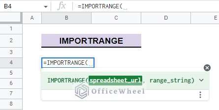

Now, let’s get back to our original task of using VLOOKUP to import data from another workbook.

Step 1: Preparing Datasets

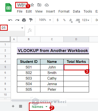
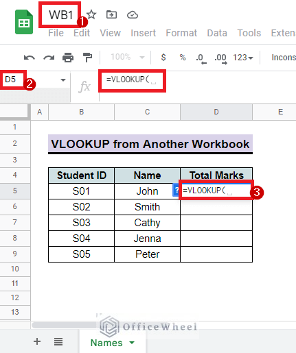
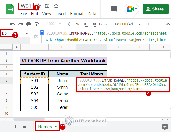
At first, to start the operation we need to prepare two different worksheets. The names of the students are in a workbook named ‘WB1’ in a sheet named ‘Names’:

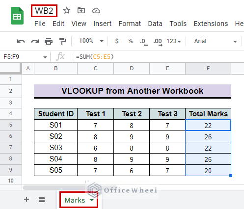
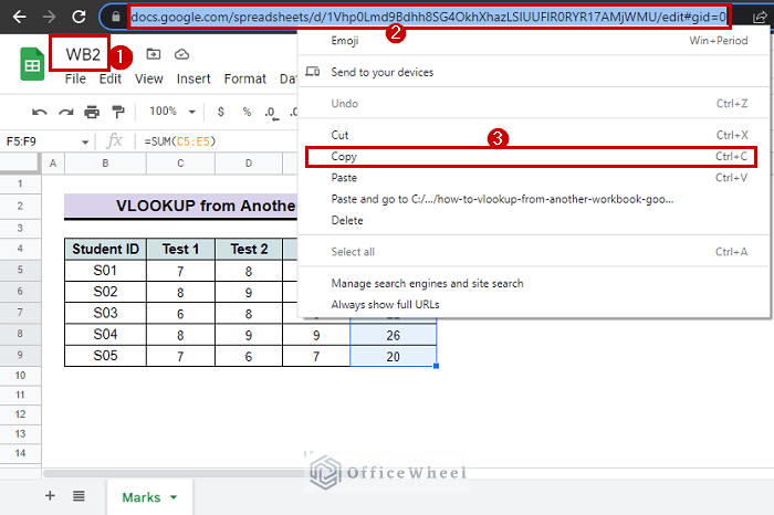
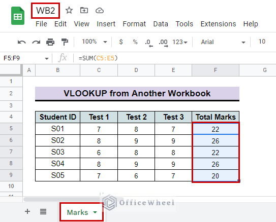
The marks obtained by the students are in a separate workbook named ‘WB2’ in a sheet named ‘Marks’:

We want to access the ‘WB2’ workbook to import marks gained by each student in the ‘WB1’ workbook and display them in cell ‘D5’ of the ‘Names’ sheet.

Step 2: Getting Started with VLOOKUP

First, click on the cell where you want the data to display. In our example cell ‘D5‘ in ‘WB1’ workbook.
After that, type in =VLOOKUP followed by the opening parentheses in the desired cell.

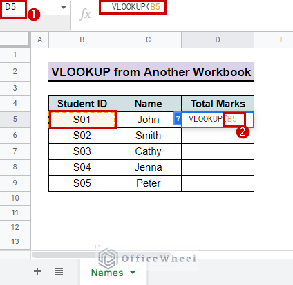
Next up, type in the value that you want to look up. For example, we type ‘B5’, followed by a comma.

Step 3: Imposing IMPORTRANGE

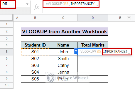
Now, For range, type in IMPORTRANGE then put in the opening parentheses.

Then, go to the workbook you want the data to import from and copy the URL of this workbook from the search bar of the browser. In our case, we open the ‘WB2’ workbook and copy the URL.

After that, go back to your main workbook and paste the URL you just copied in the formula bar after IMPORTRANGE inside a quotation. We paste the URL in ‘WB1‘ workbook It should look like this:

Similar Readings

Step 4: Importing Data Using IMPORTRANGE

Now, Put on a comma and input the name of the sheet inside from where you want to look up the value followed by opening a quotation mark followed by an exclamation mark at the end.

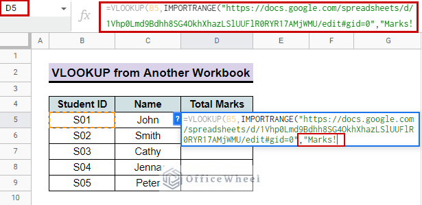
In our example it is the data is in sheet named ‘Marks‘ in ‘WB1‘ workbook. So, we type “Marks!

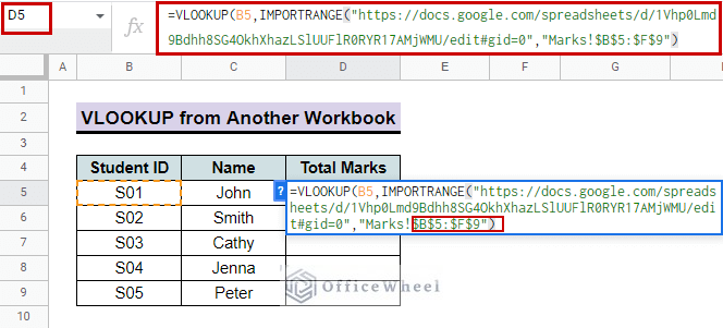
Next, type in the table range from where you want to get the data and close quotation. For our example we type in ‘B5:F9‘ then close quote. We do not want any value to change, that is why we put the $ sign in front of every row and column name to make them absolute. It looks like this: $B$5:$F$9. Then, close the parentheses for IMPORTRANGE. This is how it looks like:

Read More: Google Sheets Vlookup Dynamic Range

Step 5: Finalizing VLOOKUP

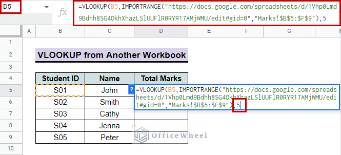
Now, Type in the column number of the table whose data you want to look up followed by a comma. For our example, we type in ‘5’ as the data is in the fifth column of the B5:F9 table.

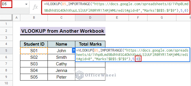
Then, type in ‘0’ as you want an exact match. Then close the parentheses. Press Enter and your data is imported from another workbook!

Step 6: Final Look

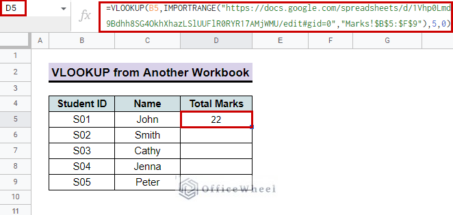
After pressing Enter our workbook looks like this:

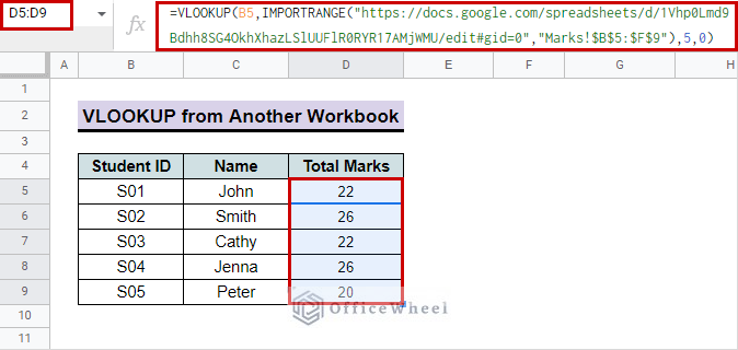
Now we copy the formula onto the next rows to get the full column of students numbers. This is how our final dataset looks:

Conclusion

In this article we showed you how to VLOOKUP data from another workbook in Google Sheets. We hope this article was useful to you to understand VLOOKUP better. Check out other articles on our site to keep on improving your Google Sheets work knowledge.

How to Use VLOOKUP to Import from Another Workbook in Google Sheets

What Is the VLOOKUP Function?

Step by Step Process of Using VLOOKUP to Import Data from Another Workbook in Google Sheets

Step 1: Preparing Datasets

Step 2: Getting Started with VLOOKUP

Step 3: Imposing IMPORTRANGE

Step 4: Importing Data Using IMPORTRANGE

Step 5: Finalizing VLOOKUP

Step 6: Final Look

Conclusion

Related Articles

Maruf Niaz

Leave a reply Cancel reply