Match Multiple Values in Google Sheets (An Easy Guide)

At a professional level, spreadsheet searches can get quite complex with the amount of varying data they might have. Thus, we have to look for viable and quick solutions for these searches that even an entry-level employee can handle. Following that train of thought, today, we will look at how to match multiple values in Google Sheets from the same column.

3 Approaches to Match Multiple Values in Google Sheets

1. Match and Return Multiple Values from a Column in Google Sheets

We start with something simple. Here we have a worksheet of Names and their respective Country of origin.

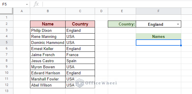
What we want to do here is we want to match each name according to their country of origin and list those names separately.

For this, we simply use the FILTER function. An advantage of the FILTER function, in this case, is that it returns values in an array by default. So, we don’t have to resort to the ARRAYFORMULA.

Our formula:

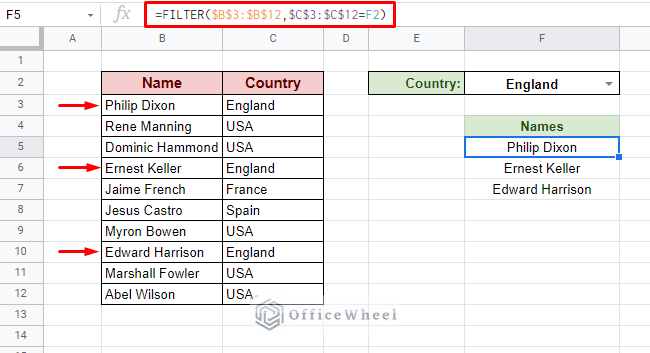
The Country column, C3:C12, contains out lookup value, and the Name column, B3:B12, contains the matched values that are to be extracted. The drop-down at cell F2 contains the criteria we are looking for.

We have also locked our cell references with absolutes ($) so that the references don’t move as we go down the range with each lookup.

Our method in action:

Read More: Match from Multiple Columns in Google Sheets (2 Ways)

2. Using REGEXMATCH to Lookup Multiple Values in Google Sheets

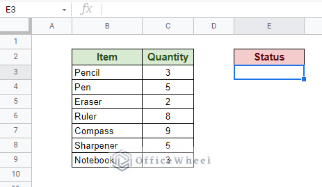
Having an item inventory is common in spreadsheet applications, and one of the major tasks involving an inventory database is lookup.

One such lookup criteria could be to match multiple conditions and return a value if TRUE.

For example, let’s say we want to know whether Pencils, Erasers, and Sharpeners are available in stock. All three must be available if we want to proceed to the next stage in shipping.

The Formula Breakdown

Since we are working with multiple text matches, the REGEXMATCH function suits this scenario perfectly.

With our three conditions, the format for REGEXMATCH would be:

Obviously, the text conditions will be enclosed within quotation marks (“”). Here we also see the biggest advantage of using REGEXMATCH, which is the ability to use regular expressions to enhance our criteria. We are using the “vertical bar” or “pipe” symbol (|) to add multiple criteria to our match case. This symbol acts as an OR logic.

So, if one of the Items listed in the formula is present in the inventory, it will return 1 (TRUE), otherwise 0 (FALSE):

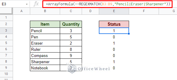
More than likely, a practical database will have varying ranges of items in the column. So, to accommodate that, we will update our formula to accept an infinitive range. Changing B3:B9 to B3:B.

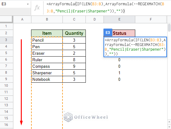
Now, for our condition to be TRUE, we must SUM the return values. Since, if the item exists in the inventory, our formula returns 1. So, if all three items are present, the sum value must be equal to or greater than 3.

Thus, our updated (and final) formula is:

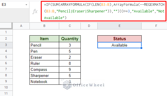
Note: The text values can be changed to cell references to make the formula more dynamic. This can be useful when looking up different combinations of items.

Read More: Use REGEXMATCH Function for Multiple Criteria in Google Sheets

Similar Readings

• Find All Cells With Value in Google Sheets (An Easy Guide)
• If Cell Contains Text Then Return Value in Another Cell in Google Sheets
• Google Sheets: Conditional Formatting with Multiple Conditions
• Conditional Formatting with Multiple Conditions Using Custom Formulas in Google Sheets
• Find Cell Reference in Google Sheets (2 Ways)

3. Using MATCH Function to Match Multiple Values

In our previous section, the core idea to match multiple values in Google Sheets revolved around using the OR logic by taking advantage of a versatile match function, REGEXMATCH.

We can take a similar approach to create a formula that will act as a direct alternative to the previous approach.

We do this by utilizing the MATCH function.

By default, the MATCH function returns the index of the matched value:

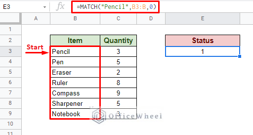
Us having three match criteria (Pencil, Eraser, and Sharpener) means that we will have three MATCH functions in an OR logic (the functions will be separated by a + symbol).

Now, to make sure that all the values exist in our range, we must return a Boolean TRUE. Since we know that if any match occurs, the MATCH function will return a value. And to make sure that all the MATCH functions are turning a value, we enclose them in an AND function.

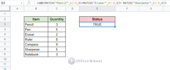
Now, to send a proper message, we utilize the IF function and finish our formula:

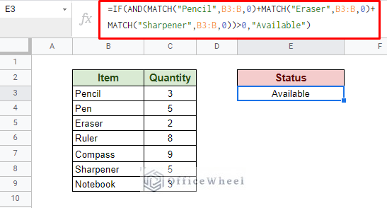
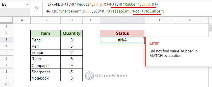
Now you might be asking: Why haven’t you included a message for the FALSE statement?

That is because, if a value does not exist in the given range, the MATCH function returns an #N/A error instead of FALSE.

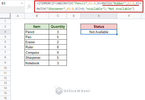
So instead, we enclose our formula within the error handling function called IFERROR.

Read More: Match Multiple Values in Google Sheets (An Easy Guide)

Final Words

That concludes all the ways we can match multiple values in Google Sheets. We hope that our methods come in handy for your spreadsheet tasks.

Feel free to leave any queries or advice you might have for us in the comments section below.

Related Articles

• IF and OR Formula in Google Sheets (2 Examples)
• How to Use VLOOKUP for Conditional Formatting in Google Sheets
• [Fixed!] INDEX MATCH Is Not Working in Google Sheets (5 Fixes)
• Use of Google Sheets INDEX MATCH in Multiple Columns
• Alternative to Use VLOOKUP Function in Google Sheets
• Using INDEX MATCH in Google Sheets – A Deep Dive
• INDEX-MATCH with Multiple Criteria in Google Sheets (Easy Guide)