When you work with a large amount of corresponding data, it is very challenging to find and reference data from different tables. In this case, the VLOOKUP or vertical lookup function in Google Sheets can automatically look up values and get relevant data from the same or different sheets. In this article, we will go through VLOOKUP for all matches in Google Sheets.
A Sample of Practice Spreadsheet
You can download spreadsheets from here and practice.
2 Handy Approaches to VLOOKUP All Matches in Google Sheets
In Google Sheets, the VLOOKUP function by default looks for a range of values and only presents the corresponding value for the first match. So, it is a good way to use the FILTER function to look up and return all matches in Google Sheets. The FILTER function will allow you to filter your dataset as per your condition or conditions. The general syntax for the FILTER function is:
=FILTER (range, condition1, [condition2, …])- range: This is the range of cells that you want to filter.
- condition1: This is the column/row that returns an array of TRUE or FALSE values. This needs to be of the same size as that of the range.
- [condition2]: This is an optional argument and can be the second condition for which you check the formula. This again can be a column/row that returns an array of TRUEs/FALSEs. This needs to be of the same size as that of the range.
Using this FILTER function, you can return all matches vertically or horizontally as per your requirement. Here, we will discuss both ways:
1. Using FILTER Function for Single Criterion
In the following examples, we will use the FILTER function to look up and match a single criterion in Google Sheets.
1.1 Return All Matches Vertically
By default, the FILTER function presents the lookup matches vertically. To do so,
Steps:
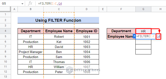
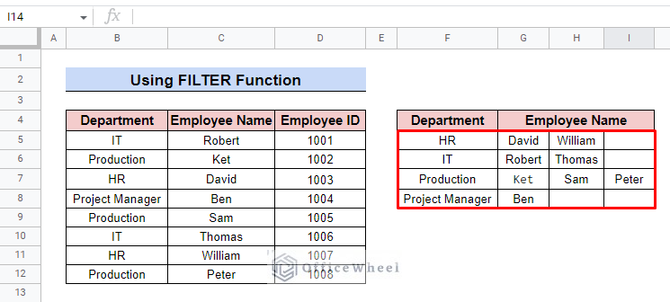
- First, you have to create a new table in the same spreadsheet which presents the search key and return values. Here, we create a new table representing Department and Employee Name.
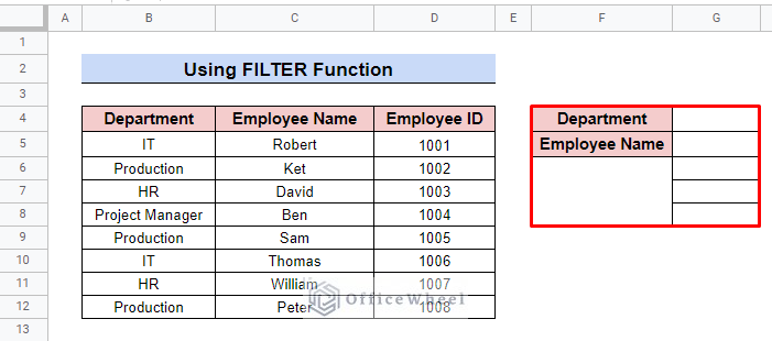
- Then enter the search key into cell G4. We will search for employees in the HR department.
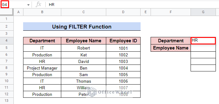
- For the return value, we enter the FILTER formula in cell G5.
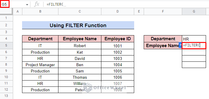
- In the function, first insert C:C column which contains the Employment Name.
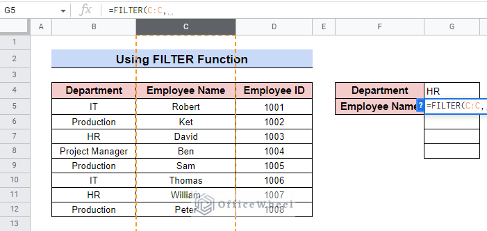
- Then enter search key cell G4.
- After that, insert B:B column in the formula.
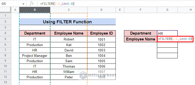
- Finally, after applying the function you can find all the matches for the search key in the same column presenting vertically.
=FILTER(C:C,G4=B:B)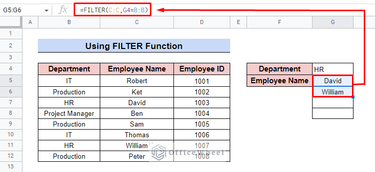
- Additionally, you can look up other departments as well by applying the formula.
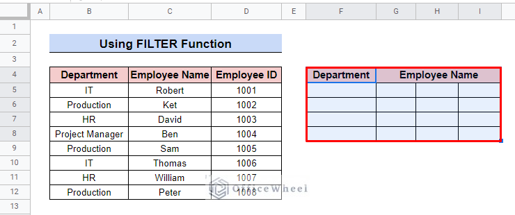
1.2 Return All Matches Horizontally
You can also return all matches horizontally in the new table. To do so, you can use the TRANSPOSE function if you want to show a vertical table horizontally.
Steps:
- First, you have to create a new table. Here, we add Department and Employee Name for the new table.
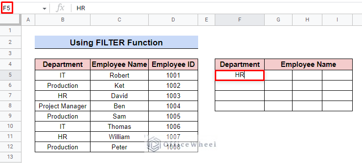
- Then insert the search key in cell F5.
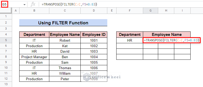
- For presenting all matches horizontally apply the formula to the G5 cell.
=TRANSPOSE(FILTER(C:C,F5=B:B))- Here, the TRANSPOSE function is used to convert the columns into rows to present the data horizontally.
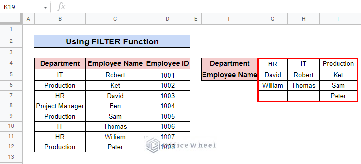
- Finally, you can find the return value displayed in horizontal form.
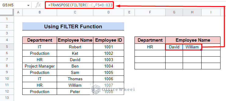
- Additionally, you can add the other departments in the same way.
Read More: Highlight Cell If Value Exists in Another Column in Google Sheets
Similar Readings
- How to Use VLOOKUP Function for Exact Match in Google Sheets
- Do Reverse VLOOKUP in Google Sheets (4 Useful Ways)
- How to Use VLOOKUP with IF Statement in Google Sheets
- VLOOKUP Multiple Columns in Google Sheets (3 Ways)
- How to Use VLOOKUP with Drop Down List in Google Sheets
2. Applying Multiple Criteria
You can use these VLOOKUP formulas for multiple criteria as well. It is applicable when you have two or more common fields in two tables. For multiple criteria, we first have to add a helper column in our dataset. To do so,
Steps:
- First, add a new column in the first dataset to apply VLOOKUP for multi-criteria and name it. Here, we name the column Dpt & Emp_Name.
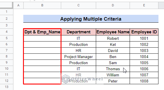
- Then insert the formula to join two columns.
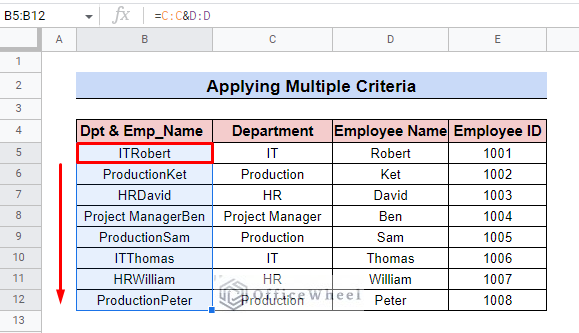
=C:C&D:D- Here, C:C represents Department and D:D represents Employee Name.
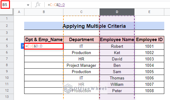
- After that, use the fill handle to fill the column.
- Now, below the first table, we will create a new table where the Department and Employee Name columns are common. We are looking for the Employee ID.
- Enter the VLOOKUP formula in cell E16.
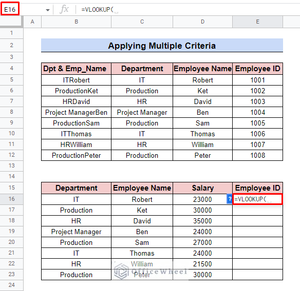
- Now, go to the new table and insert the VLOOKUP function for Employee ID. In these two tables, the Department and Employee Name are the common columns.
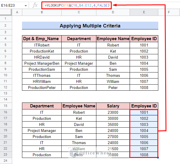
=VLOOKUP(B16&C16,B4:E12,4.FALSE)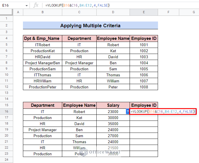
Formula Breakdown
- B16&C16 is the search key.
- B4:E12 represents the entire dataset or the range of the table.
- 4 is the column number for the new table where we want to apply the VLOOKUP function.
- FALSE is used to indicate the exact value.
- To get values for the entire column use the fill handle.
Read More: How to VLOOKUP with Multiple Criteria in Google Sheets
Limitation of Using VLOOKUP Function to Find Multiple Matches in Google Sheets
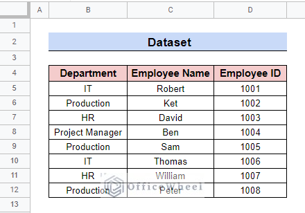
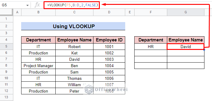
To apply the VLOOKUP function here, we have a dataset representing two columns: Department, Employee Name, and Employee ID.
If you want to develop another table containing only Employee ID and their Department, you can use the VLOOKUP function to extract the department by using the Employee ID.
The general syntax:
=VLOOKUP(search_key, range, index, [is_sorted])For the dataset, the function is:
=VLOOKUP(F5,B:D,2,FALSE)Finally, you can see the result in your newly created table in cell G5.
Formula Breakdown
- Here, F5 is the search key cell that we want to search.
- B:D represents the entire dataset or table.
- 2 is the column number from where the data will be extracted. Employee Name is the second column on our data range.
- We use FALSE to get the exact value.
As you can see, the VLOOKUP function does not show all the matches at the same time, rather it shows only the first matching value. That’s why to show all the matches we use the FILTER function.
Read More: How to VLOOKUP Last Match in Google Sheets (5 Simple Ways)
Things to Remember
- You can use VLOOKUP to find a single match only.
- Insert the range carefully in the FILTER function.
- Always use the fill handle to apply the function to the entire column.
Conclusion
I hope these methods mentioned above will now assist you to use VLOOKUP for all matches in Google Sheets. So, feel free to comment when you have any queries related to this article. Or you may take a look at our different articles associated with Google Sheets VLOOKUP on our OfficeWheel website.
Related Articles
- How to Use VLOOKUP with Named Range in Google Sheets
- Google Sheets Vlookup Dynamic Range
- How to Use Nested VLOOKUP in Google Sheets
- [Fixed!] Google Sheets If VLOOKUP Not Found (3 Suitable Solutions)
- How to VLOOKUP for Partial Match in Google Sheets
- Create Hyperlink to VLOOKUP Cell in Multiple Rows in Google Sheets
- How to Use IFERROR with VLOOKUP Function in Google Sheets
- VLOOKUP Between Two Google Sheets (2 Ideal Examples)