Nowadays, we frequently use INDEX MATCH to find a value in a dataset. It offers us a lot of benefits than using the VLOOKUP function. The VLOOKUP function only searches for values on the right side of the dataset. But the combination of INDEX and MATCH functions can search on both sides of a dataset. Nevertheless, there are also drawbacks. In Google Sheets, INDEX MATCH occasionally returns an incorrect value. This can happen due to various reasons. In this article, we’ll see 5 useful solutions when INDEX MATCH is not working in Google Sheets with clear images and steps. At last, you’ll get an output like the following image.
A Sample of Practice Spreadsheet
You can download Google Sheets from here and practice very quickly.
5 Useful Fixes When INDEX MATCH Is Not Working in Google Sheets
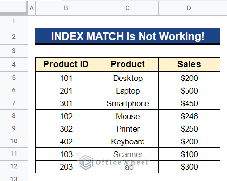
Let’s get introduced to our dataset first. Here we have some product ids in Column B, products in Column C, and their sales prices in Column D. We will try to use INDEX MATCH to look up a value in this dataset and find out that INDEX MATCH is not working. So, I’ll show you 5 useful solutions when INDEX MATCH is not working in Google Sheets by using this dataset.
Solution 1. Inserting Search Type Correctly
If you don’t specify the right search type in the formula, INDEX MATCH won’t return the right value. There are 3 types of search type values for the MATCH function. They are described below:
- 0: When the data range is not sorted, it denotes an exact match and is used.
- 1: We use it when the data range is sorted in ascending order. It returns the largest value less than or equal to the search key.
- -1: We use it when the data range is sorted in descending order. It gives the smallest value greater than or equal to the search key.
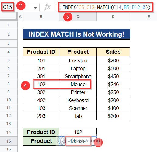
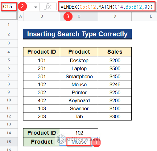
Our dataset is not sorted. So, when you utilize the formula, you must supply an exact match meaning you have to use 0 in your formula. Let’s say we wish to use the product id number in Cell C14 to get the name of the product in Cell C15. The product will immediately be updated if we modify the product id. For that purpose, we have written the formula below:
=INDEX(C5:C12,MATCH(C14,B5:B12))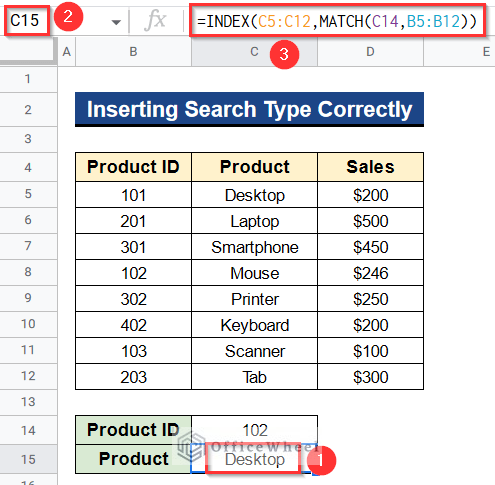
In this instance, the formula ought to have found Mouse in Cell C15. However, Desktop was displayed, which is the incorrect value. This is because we omitted the search type number, and so it considered the search type 1 by default, which returned output for the closest search value 101. Thus, it provides an incorrect response. Let’s follow the steps below to return the right value.
Steps:
- Firstly, select Cell C15.
- Secondly, type the new formula instead of the previous one-
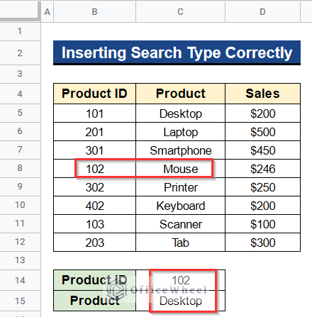
=INDEX(C5:C12,MATCH(C14,B5:B12,0))- Then, hit Enter to see the correct result.
Formula Breakdown
- MATCH(C14,B5:B12,0)
First of all, this function search for the product id of Cell C14 in the range from Cells B5 to B12 in the dataset and gives its position.
- INDEX(C5:C12,MATCH(C14,B5:B12,0))
Then, the INDEX function gives the corresponding product by matching it with the product id it gets from the MATCH function.
- Finally, you’ll see that the product id and product are matching with the dataset. Because this time we have inserted the search type number correctly in our formula.
Read More: INDEX-MATCH with Multiple Criteria in Google Sheets (Easy Guide)
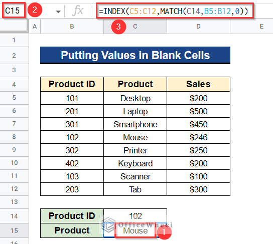
Solution 2. Putting Values in Blank Cells
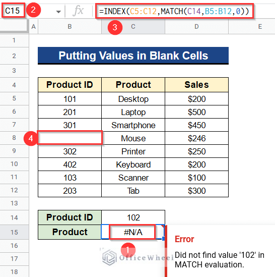
If we have blank cells inside the range of the dataset, we may see the wrong value in the desired cell. In the picture below, we have put the following formula in Cell C15–
=INDEX(C5:C12,MATCH(C14,B5:B12,0))But it is giving a #N/A error because there is a blank cell in Column B. The product id number 102 is missing from Column B, so the INDEX MATCH isn’t finding the product. Follow the steps below to put the value in the blank cell.
Steps:
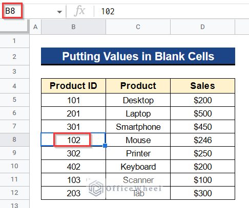
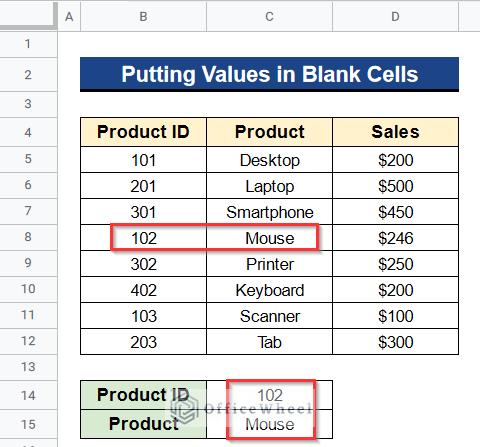
- At first, put 102 into Cell B8.
- Then, insert the following formula in Cell C15–
=INDEX(C5:C12,MATCH(C14,B5:B12,0))- To show the right answer, press Enter after that.
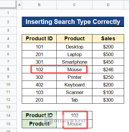
- At last, the product id and product will match with the dataset, as you can see. Because we filled in the blank cell this time with a value.
Read More: Find All Cells With Value in Google Sheets (An Easy Guide)
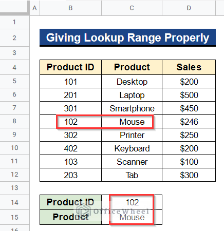
Solution 3. Giving Lookup Range Properly
The INDEX MATCH will not give the correct result if the wrong lookup range is provided. To understand the problem, take a look at the picture below. Here, we used the formula below in Cell C15–
=INDEX(C5:C12,MATCH(C14,D5:D12,0))Here, the formula is showing the #N/A error in Cell C15 in the following picture because we provided the wrong lookup range. We put Cells D5 to D12 as our range which are the sales value.
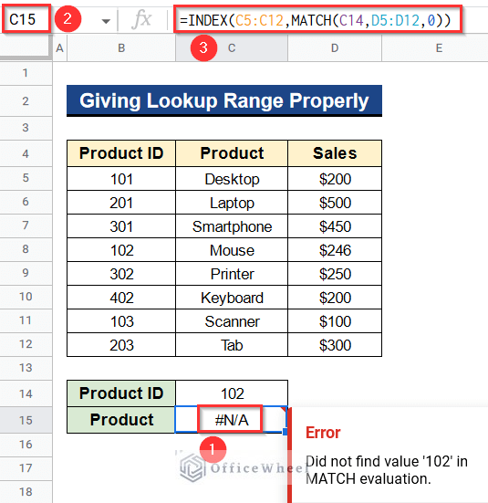
So, we have to put Cells B5 to B12 as our lookup range which are the product ids. You’ll find the steps below to get the correct result.
Steps:
- In the first place, select Cell C15 and type the formula with the correct lookup range-
=INDEX(C5:C12,MATCH(C14,B5:B12,0))- Then, hit Enter to see the result.
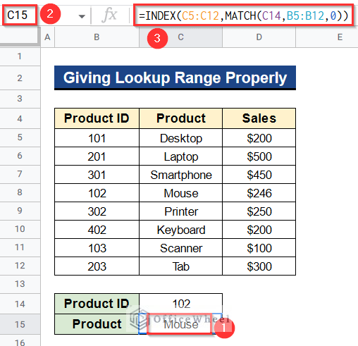
- Ultimately, as we provided the proper lookup range, the product id, and product will match with the dataset.
Similar Readings
- Google Sheets Conditional Formatting with INDEX-MATCH
- How to Create Conditional Drop Down List in Google Sheets
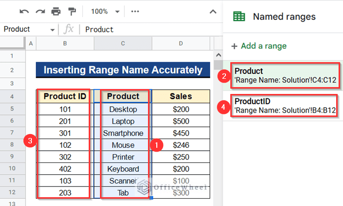
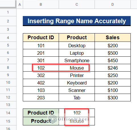
Solution 4. Inserting Range Name Accurately
When you are using predefined Named Ranges in your formula in Google Sheets, you need to be extra careful. We have the product in Column C so we named it Product by using the Named Ranges feature of Google Sheets. We do the same for Column B which has product ids.
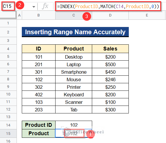
After that, when we are putting the following formula using the named ranges in Cell C15, it is giving us the incorrect result-
=INDEX(ProductID,MATCH(C14,ProductID,0))This happened because we put the wrong range name in our formula. It should be Product instead of ProductID in the INDEX function. The solution is given below.
Steps:
- In the beginning, insert the following formula in Cell C15–
=INDEX(Product,MATCH(C14,ProductID,0))- Then, press Enter to get the correct result.
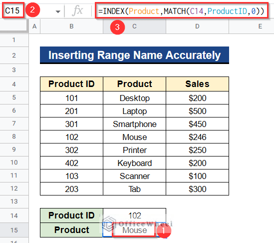
- In the end, the product id and product will match with the dataset because we specified the correct range name.
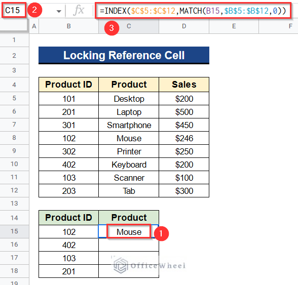
Solution 5. Locking Reference Cell
We have to lock the reference cells when we drag the INDEX MATCH formula down or across for multiple search values. Below, we have used the following formula for multiple IDs-
=INDEX(C5:C12,MATCH(B15,B5:B12,0))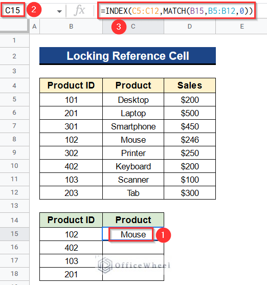
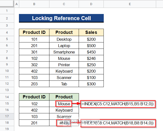
Then, we dragged the formula down in the picture below. We can see the correct results in Cells C15 to C17 but with errors. And in Cell C18, we can see the #N/A error. This happens when your reference is not locked. The arrays will move along the direction of the dragging and produce wrong results or errors. To get rid of the problem, you need to lock your reference. In Google Sheets, we use the Dollar Sign ($) to lock any cell or reference.
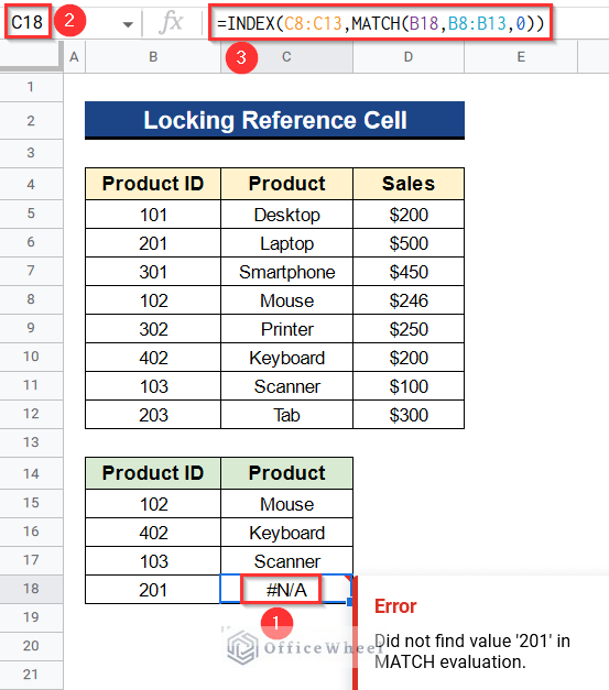
You can see in the following picture that the range is changed because we don’t lock the reference cells properly. That’s why it is showing the #N/A error. Let’s follow the steps below to learn this solution.
Steps:
- Before all, type the following formula in Cell C15 with the Dollar Sign ($)–
=INDEX($C$5:$C$12,MATCH(B15,$B$5:$B$12,0))- Then, hit Enter to get the output.
- After that, apply the Fill Handle tool to use the formula in the rest of the cells of Column C.
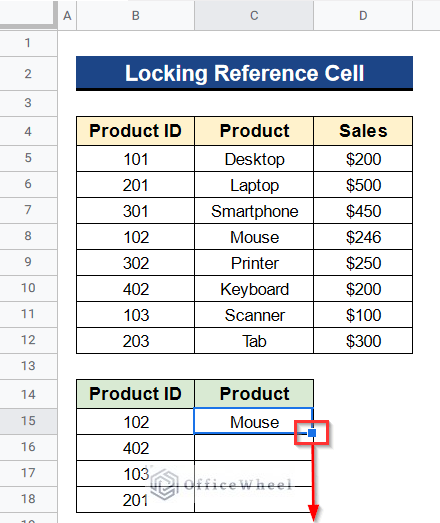
- Finally, you’ll see that all the product ids are matching with the products perfectly.
Read More: Find Cell Reference in Google Sheets (2 Ways)
Things to Remember
- When you have a small dataset, INDEX MATCH issues are fairly simple to solve.
- However, you must exercise caution while working with a huge dataset.
- You must first identify the issue within your dataset before applying the appropriate solution.
Conclusion
That’s all for now. Thank you for reading this article. In this article, I have discussed 5 useful solutions when INDEX MATCH is not working in Google Sheets. Please comment in the comment section if you have any queries about this article. You will also find different articles related to google sheets on our officewheel.com. Visit the site and explore more.