INDEX-MATCH with Multiple Criteria in Google Sheets (Easy Guide)

We are already aware of how powerful the INDEX-MATCH combination is when extracting data in Google Sheets. If not, please visit our Using INDEX MATCH in Google Sheets – A Deep Dive article to familiarize yourself. But in this article, we will take things a step further and see how to  use INDEX-MATCH with multiple criteria in Google Sheets

Let’s get started!

How to Use INDEX MATCH with Multiple Criteria in Google Sheets

To show our example, we will use the following worksheet:

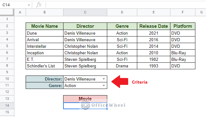
Here we have a small section of a database of movies. And underneath that, we have our conditions or criteria, which in this case are the Director Name and Genre.

The criteria will be used to extract the name of the movie.

For multiple criteria INDEX-MATCH, we have the following formula syntax:

Formula breakdown:

We will start from the inside then move outward.

• MATCH: The function returns the position of the matching criteria.
  • 1: This is the fixed search key.
  • (criteria_1)*(criteria_2)*…(criteria_N): Our multiple criteria/conditions. The asterisk (*) acts as the AND logic to combine all criteria into one match condition.
  • 0: Defines that we are looking for an exact match, making this our fixed search type.
• INDEX: Retrieves a value from a given range according to row and column reference.
  • reference_range: The cell range of the values that will be returned if there is a match.

Thus, our formula to extract the Movie name according to the given criteria will be:

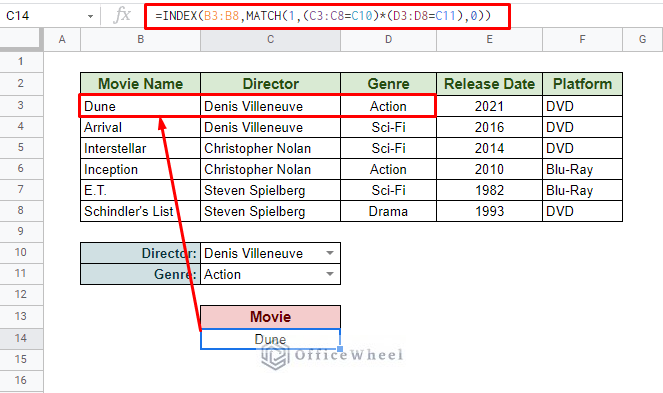
We can try it for different conditions:

But what happens if we give a condition that does not exist in our dataset?

The simple answer is this:

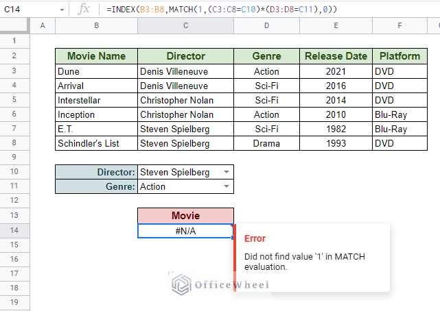
We get a #N/A error.

To overcome this error, we will replace it with a message. This can be achieved by the IFERROR function.

So our modified formula becomes:

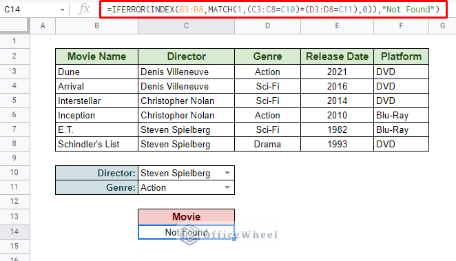
In the instance of an error, the IFERROR function will return a meaningful message.

Read More: Use of Google Sheets INDEX MATCH in Multiple Columns

An Alternative Approach

Instead of using the asterisk (*), we can also use the ampersand (&) to concatenate our criteria. But in doing so, we must bring a couple of modifications to our INDEX-MATCH formula.

Thus, our updated formula becomes:

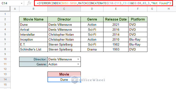
Formula Breakdown:

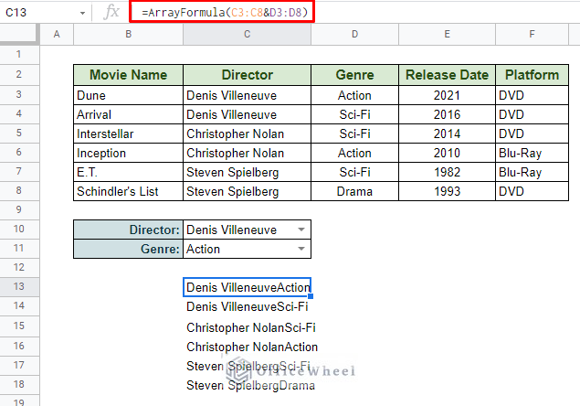
C3:C8&D3:D8: Combines all the criteria instance rows into one so that it can be used in MATCH. The output is presented as an array of all the rows.

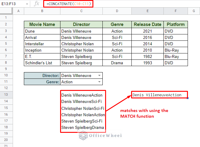
CONCATENATE(C10:C11): Combines the criteria into one value to help check against all instances in the MATCH function.

The rest of the function remains the same as discussed in the previous section.

As you have seen in our formula breakdown, we have used ARRAYFORMULA to enclose our formula to present the values of all the instances as an array. We can do the same for the final INDEX-MATCH formula, actually, it is recommended that you do so.

So, instead of pressing ENTER to input the formula, press CTRL+SHIFT+ENTER to automatically present your formula as an array. Or you can just manually input it.

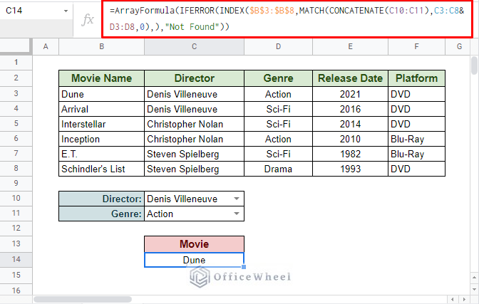
Final Words

That concludes all the ways we can use INDEX MATCH with multiple criteria in Google Sheets. While we have shown our examples with only two criteria, the formula allows us to use much more than that.

We hope that our discussion helped you understand the potential of INDEX-MATCH better and why, for some cases, it is better than VLOOKUP.

Feel free to leave any queries or advice you might have for us in the comments section below.

Related Articles

• [Fixed!] INDEX MATCH Is Not Working in Google Sheets (5 Fixes)
• Google Sheets Conditional Formatting with INDEX-MATCH
• Use INDEX MATCH Across Multiple Sheets in Google Sheets
• Combine VLOOKUP and HLOOKUP Functions in Google Sheets
• Alternative to Use VLOOKUP Function in Google Sheets
• How to Create Conditional Drop Down List in Google Sheets
• Match Multiple Values in Google Sheets (An Easy Guide)
• Find Cell Reference in Google Sheets (2 Ways)