How to Create Conditional Drop Down List in Google Sheets

Imagine you have a dataset containing several categories of products. Each category contains various unique products. Now you need to create a dropdown list for your customers to choose a particular product category followed by their desired product from that category. How can you do that? Well, you can easily create a conditional drop down list in Google Sheets to get the desired result. Follow the article to learn several ways to do that in Google Sheets.

A Sample of Practice Spreadsheet

What Is Conditional Drop Down List?

In Google Sheets, a dropdown list is very useful to select a particular value from a list of options. This works only for a single list of values or options. Suppose you are working with 2 dropdown lists. The 2nd dropdown list is dependent on the option selected in the 1st dropdown list. Then the 2nd one is a conditional dropdown list.

For example, assume the 1st dropdown list contains ‘Smartphone’ and ‘Computer’. If you select Smartphone, then the 2nd dropdown list will contain Samsung, Apple, and Huawei. If you select Computer, then the 2nd dropdown list will contain Acer, Dell, and HP. You can create multiple conditional dropdown lists in Google Sheets to choose the desired option that meets all the criteria.

4 Ways to Create Conditional Drop Down List in Google Sheets

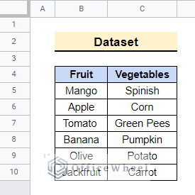
The dataset below contains some names of Fruit and Vegetables. First, we will create a drop-down list using this dataset to be able to choose between Fruit and Vegetables. Then we will create a conditional dropdown list to be able to select a particular fruit or vegetable depending on the selection in the 1st dropdown list.

Here, we are going to learn 4 ways to create the conditional drop down list in Google Sheets. So, let’s start doing that.

1. Applying FILTER Function

We can use the FILTER Function to create a conditional drop down list. This function allows us to filter data based on the specified criteria. Follow the steps below to learn how to do it.

📌 Steps:

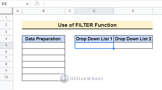
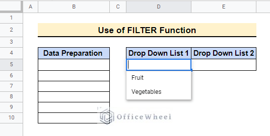
• Here we will create a drop-down list in cell D5 showing Fruit and Vegetables. After that, we will create another drop-down list in cell E5 showing the individual items. So, first, select cell D5.

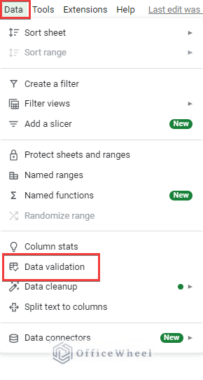
• Then select Data >> Data Validation as shown below. After that, the Data validation window will pop up.

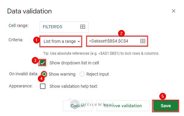
• Then select List from a range as the criteria and choose the range B4:C4 from the Dataset sheet. Lock the cell references so that the values don’t change.
• Next check the “Show dropdown list in cell” checkbox. You may select the radio button for Show warning or Reject input to avoid invalid data entry. Then click on Done.

• After that, the drop-down list will be created as follows.

• Before creating the conditional drop-down list, enter the following formula in cell B5 as shown below.

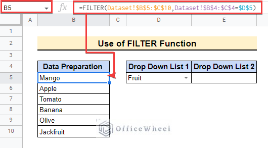
• Here, Dataset is the sheet name. The formula filters range B5:C10 in that sheet if cell D5 i.e Drop Down List 1 matches the range B4:C4 in that sheet.
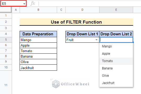
• Now you can create the conditional dropdown list in cell E5 by applying Data validation as earlier using the range B5:B10.

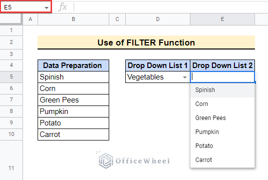
• If you select Vegetables in Drop Down List 1, then the conditional drop down list will look as follows.

Read More: Create Drop Down List in Google Sheets from Another Sheet

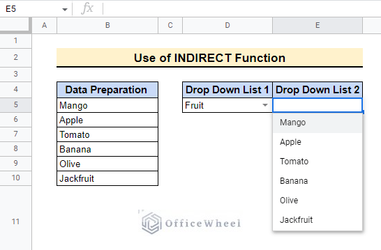
2. Using INDIRECT Function

We can also use the INDIRECT function with Named ranges to create the conditional drop down list. Let’s see how to do it.

📌 Steps:

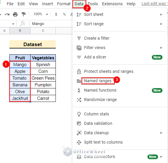
• First select cell D5 and create Drop Down List 1 as before. Then select the range B5:B10 in the Dataset sheet and go to Data> Named Ranges.

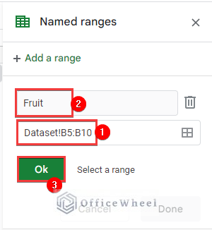
• Next, enter Fruit as the name for that range and click OK.

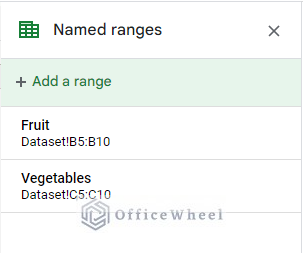
• After that, create another named range for the C5:C10 range in that sheet.

• Then insert the following formula into cell B5 and lock the cell reference by pressing F4.

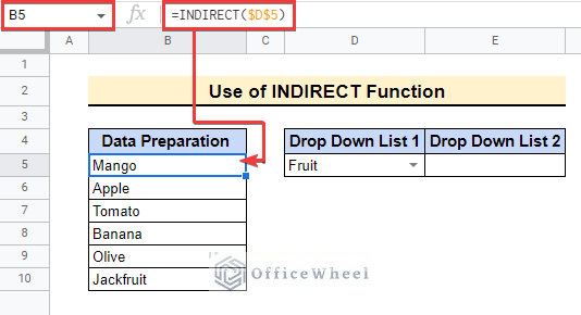
• Now you can create the conditional dropdown list in cell E5 by applying Data validation as earlier using the range B5:B10.

Read More: Create Drop Down List for Multiple Selection in Google Sheets

Similar Readings

• How to Remove Data Validation in Google Sheets
• Dependent Drop Down List for Entire Column in Google Sheets
• How to Add Color to Drop Down List in Google Sheets (Easy Steps)
• [Fixed!] INDEX MATCH Is Not Working in Google Sheets (5 Fixes)

3. Utilizing INDEX and MATCH Functions

Here, we will learn about utilizing the INDEX and MATCH functions to get the same result. Follow the below steps to be able to do that.

📌 Steps:

• First select cell D5 and create Drop Down List 1 as earlier.
• Then, apply the following formula in cell B5 as shown below.

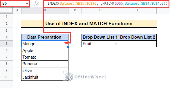
• Here the [row] input for the INDEX function is empty to return all rows of data. The MATCH function returns the [column] input for the INDEX function.
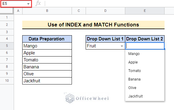
• Now you can create the conditional dropdown list in cell E5 by applying Data validation as earlier using the range B5:B10.

Read More: How To Lock Rows In Google Sheets (2 Easy Ways)

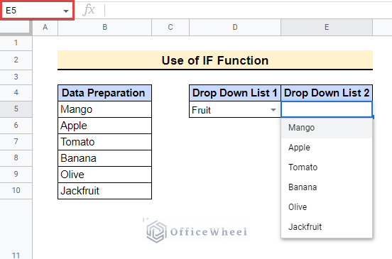
4. Applying IF Function

Finally, we will use the IF function to create an array formula to get the same result as in the earlier methods. Follow the steps below to be able to do that.

📌 Steps:

• First select cell D5 and create Drop Down List 1 as earlier.
• After that, enter the following formula in cell B5 to get the contents for the conditional dropdown list i.e. Drop Down List 2.

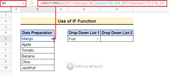
• Here the IF function has been used twice to return the range Dataset!B5:B10 or Dataset!C5:C10 based on the selection in Drop Down List 1.
• Finally, you can create the conditional dropdown list in cell E5 by applying Data validation as earlier using the range B5:B10.

Read More: How to Edit Drop-Down List in Google Sheets

Things to Remember

• You need to create Named Ranges using the INDIRECT function to create the conditional dropdown list.
• Don’t forget to lock the cell references in the formulas to avoid data missing or data mismatch issues.

Conclusion

In this article, we have shown 4 different methods to create a conditional drop down list in Google Sheets. Now you can implement the methods to create the conditional dropdown lists using your own datasets. Please let us know in the comment section if you have any queries or suggestions. You may also visit our OfficeWheel blog to explore more Google Sheets-related articles.

Related Articles

• How to Insert a Drop-Down List in Google Sheets (2 Easy Ways)
• Create Multiple Dependent Drop Down List in Google Sheets
• How to Edit Data Validation in Google Sheets (With Easy Steps)
• Multi Row Dynamic Dependent Drop Down List in Google Sheets
• How to Use Data Validation in Google Sheets from Another Sheet
• Updating Cell Values Based on Selection in Drop Down List in Google Spreadsheet
• INDEX-MATCH with Multiple Criteria in Google Sheets (Easy Guide)
• Using INDEX MATCH in Google Sheets – A Deep Dive