Google Sheets is a powerful tool for organizing and analyzing data. One of the most important features of Google Sheets is the use of formulas to perform various calculations. In some cases, you may need to add parentheses to your formulas or data to change the order of operations and ensure the correct calculation of results. In this article, we will explain how to add parentheses in Google Sheets.
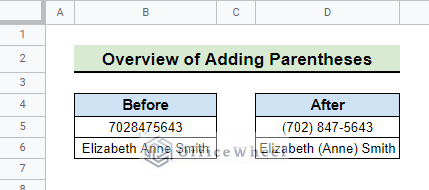
The above screenshot is an overview of the article, representing how to add parentheses in Google Sheets.
A Sample of Practice Spreadsheet
You can download the spreadsheet and practice the techniques by working on it.
5 Ideal Scenarios to Add Parentheses in Google Sheets
Parentheses are a powerful tool to control the order of operations in Google Sheets formulas. By using parentheses, you can avoid errors in your calculations.
1. Type in Parentheses Alongside Data
We use parentheses mostly in formulas in Google Sheets. We can also use parentheses with text and data to differentiate between data or texts.
The easiest way to insert parentheses in Google Sheets is by using the bracket key in your keyboard. Just simply press the SHIFT+9 keys for opening parenthesis and SHIFT+0 for closing parenthesis.
Let’s see some applications:
I. With Text
The easiest method to add parentheses in google sheets in Google Sheets is to insert them into the same cell as the text. We have a dataset with Employee ID and Employee Names. The names have three parts: first, middle, and last name.
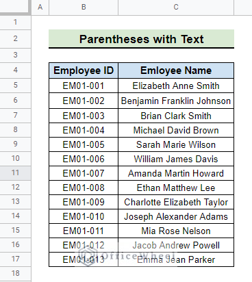
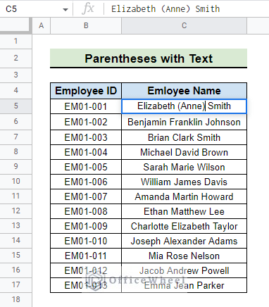
We can type in parentheses to differentiate between the first, middle, and last names.
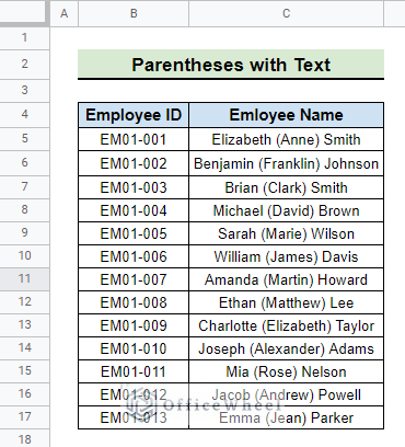
This is how the final range looks after adding parentheses to differentiate between the first, middle, and last names:
II. With Numbers
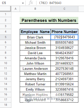
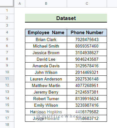
You can easily add parentheses with numbers to differentiate between numbers. In the following example, we have a dataset with phone numbers. But we can not understand the area code easily.
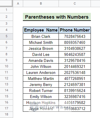
To overcome this, we can add parentheses to separate the area code from the rest of the phone numbers.
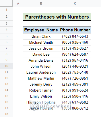
This is how the final range looks after adding parentheses to separate the area code from the rest of the phone numbers.
III. With Mathematical Calculations
In Google Sheets, parentheses determine the order of performing calculations. The order of mathematical calculations in Google Sheets is based on the PEMDAS (Parentheses, Exponents, Multiplication and Division, and Addition and Subtraction) principle.
Without Parentheses
When we do not use parentheses in a calculation, the operations are performed from left to right. For example, consider the following calculation:
=2+3*4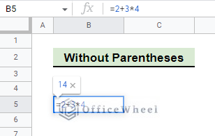
In this calculation, 3*4 is calculated first, resulting in 12. Then, 2+12 is calculated, resulting in 14. The final result is 14.
With Parentheses
But when we use parentheses in calculations, the calculation within the parentheses is performed first. For example, consider the following calculation:
=(2+3)*4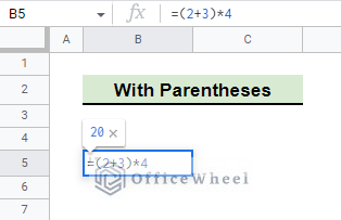
In this calculation, the calculation within the parentheses (2+3) is performed first, resulting in 5. Then, 5*4 is calculated, resulting in 20. The final result is 20.
Multiple Parentheses
It is important to use parentheses in complex calculations to ensure the accuracy of the final result. For example, consider the following calculation without parentheses:
=2+3*4/2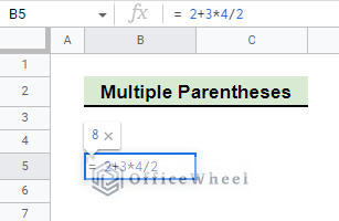
In this calculation, 3*4 is calculated first, resulting in 12. Then, 12/2 is calculated, resulting in 6. Finally, 2+6 is calculated, resulting in 8. The final result is 8.
However, if we use parentheses we can ensure the desired order of operations in the same calculation:
=(2+3)*(4/2)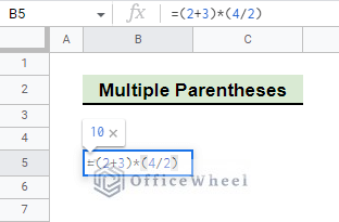
In this calculation, (2+3) is calculated first, resulting in 5. Then, (4/2) is calculated, resulting in 2. Finally, 5*2 is calculated, resulting in 10. The final result is 10.
Nesting Parentheses
Nesting parentheses refer to the use of multiple sets of parentheses within a single calculation.
For example, consider the following calculation:
=((2+3)*4)+5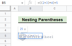
In this calculation, the innermost set of parentheses (2 + 3) is calculated first, resulting in 5. Then, 5 * 4 is calculated, resulting in 20. Finally, 20 + 5 is calculated, resulting in 25. The final result is 25.
Read More: How to Insert Equation in Google Sheets (4 Tricky Ways)
2. Wrap Negative Numbers in Parentheses
We begin by asking ourselves the question:
Why is It Necessary to Wrap Negative Numbers in Parentheses?
Wrapping negative numbers in parentheses in Google Sheets is necessary for various different reasons. That include:
- Enhance the clarity of data.
- Improve readability of large datasets.
- Increase data accuracy.
- Reduce mistakes.
Here are some ways we can go about achieving this:
I. Setting Financial Number Format
The financial number format in Google Sheets allows you to arrange your numbers to make them easier to read and understand.
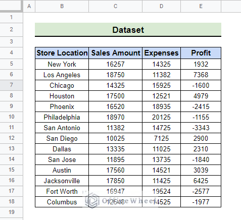
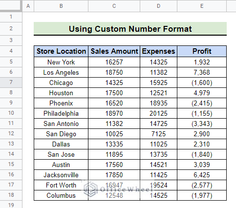
We have a dataset with the Store Locations of a company, with their Sales Amount, Expenses, and Profit in a particular month. The data in the Profit column may be a negative, indicating loss for that particular month.
Steps:
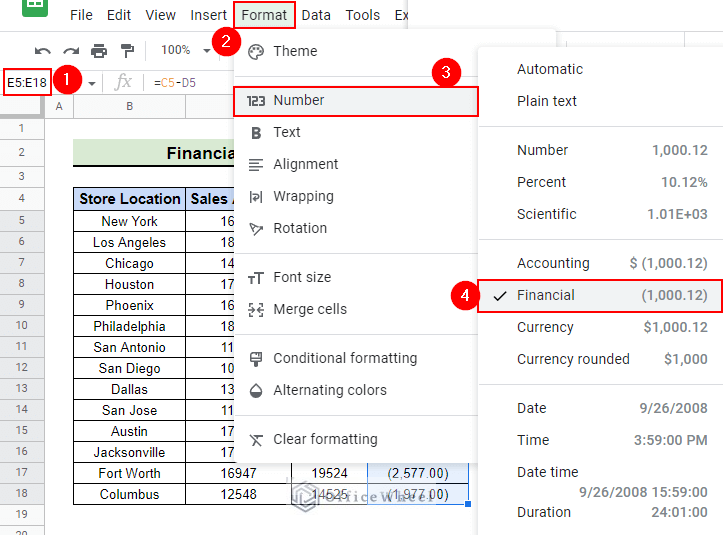
- First, select the cells where the numbers are located and go to Menu bar > Format > Number > Financial. We select the range E5:E18 for our example.
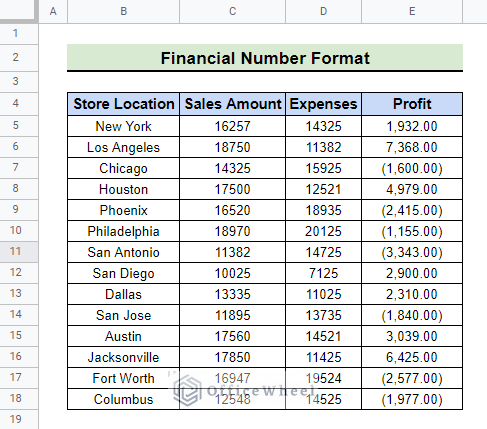
- The financial number format has been applied to the numbers, displaying negative values within parentheses.
II. Using Custom Number Format
The financial number format displays the negative numbers in parentheses. However, this format may include additional features that you may not prefer. Therefore, a custom number format may be a more suitable option for you to consider. For this method, we use the same dataset we used in the previous method.
Steps:
- First, select the cells where the numbers are located and go to Menu bar > Format > Number > Custom number format. We select the range E5:E18 for our example.

- Next, you will see a Custom number formats dialogue box appear.
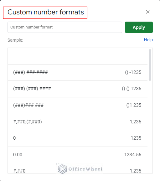
- Type the following custom number format in the dialogue box and click on Apply to apply the custom format:
#,##0;(#,##0)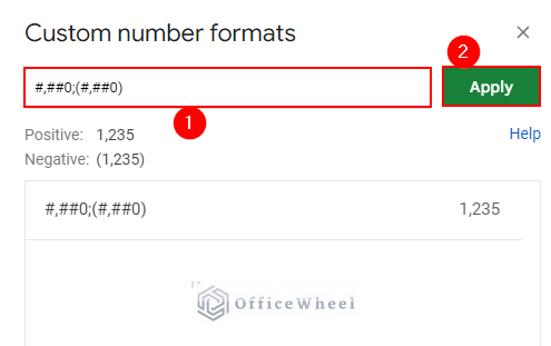
The first part of the format, #,##0, is for the positive numbers. The second part, (#,##0) is for the negative numbers. The semicolon(;) separates the parts to create a custom number format. The # symbol is used to represent a digit placeholder, while the 0 represents zero.
- Finally, the custom format is applied to the selected cells.
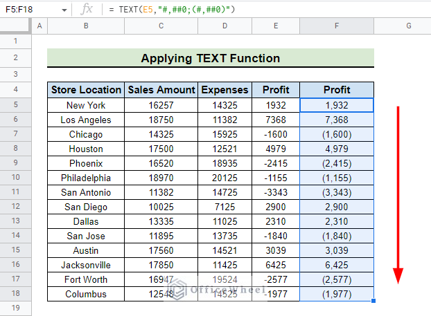
III. Applying TEXT Function
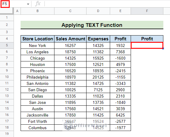
The TEXT function can be used to display negative numbers in parentheses. The TEXT function transforms a numerical value into a text representation based on a given format. We use the same dataset we used in the previous methods.
Steps:
- First, go to the cell where you want to display the number. We go to cell F5 in our example.
- After that, type the following formula:
= TEXT(E5,"#,##0;(#,##0)")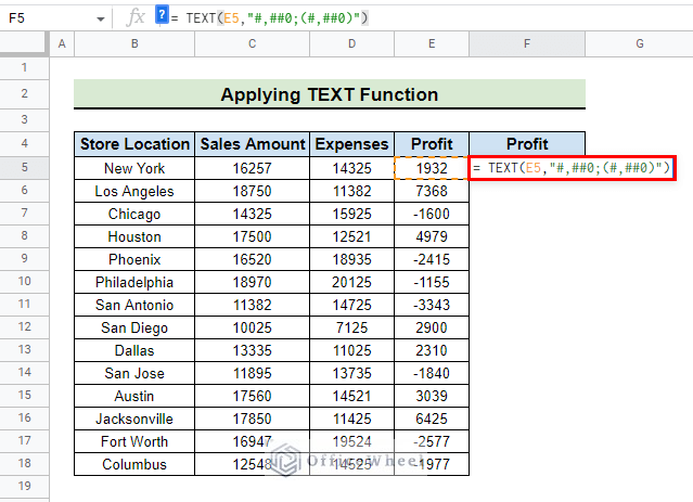
Formula Explanation:
TEXT(E5,”#,##0;(#,##0)”)
- The TEXT function takes the value in cell E5 and formats it according to the format #,##0;(#,##0).
- #,##0;(#,##0) consists of two parts separated by a semicolon (;). The part before the semicolon represents the format for positive numbers, while the part after the semicolon represents the format for negative numbers.
- Then, press ENTER to display the numbers according to the format. Use autofill to copy the formula to the cells below.
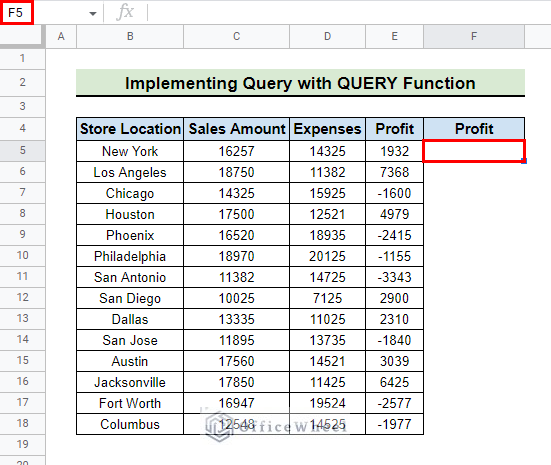
IV. Implementing Query with QUERY Function
The QUERY function in Google Sheets allows you to arrange data in a table-like format by writing a query. One of the many things you can do with the QUERY function is to format negative numbers in parentheses. We use the same dataset we used in the previous methods.
Steps:
- First, go to the cell where you want to apply the formula. We go to cell F5 in our example.
- After that, type the following formula:
=QUERY(E5:E18,"SELECT E FORMAT E '#,##0;(#,##0)'")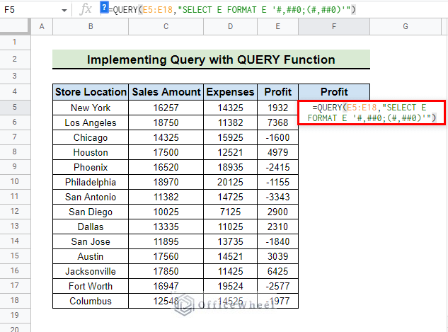
Formula Explanation:
QUERY(E5:E18,”SELECT E FORMAT E ‘#,##0;(#,##0)'”)
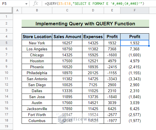
- The QUERY function will select the range E5:E18 to format.
- SELECT E selects the values in column E.
- FORMAT E ‘#,##0;(#,##0)’ applies the number format to the selected range.
- #,##0;(#,##0) specifies the number format.
- Finally, press ENTER to display the numbers according to the specified format.
Read More: How to Insert Formula in Google Sheets for Entire Column
Similar Readings
- How to Insert Video in Google Sheets (2 Easy Ways)
- Insert Multiple Columns in Google Sheets (2 Quick Ways)
- How to Insert an Exponent in Google Sheets (3 Easy Ways)
- Insert a Calendar in Google Sheets (2 Effective Ways)
- How to Insert Multiple Rows in Google Sheets (4 Ways)
3. Customize Phone Numbers by Adding Parentheses
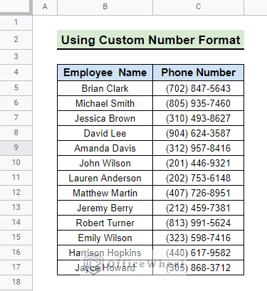
Customizing phone numbers with parentheses can help to separate the area code from the rest of the phone numbers. This makes it easier to read.
I. Using Custom Number Format Feature
You can easily customize phone numbers using a custom number format to separate the area code from the rest of the phone numbers. We have a dataset with some Employee Names and Phone Numbers. We will use this dataset to separate the area code from the rest of the phone numbers.
Steps:
- First, select the cells where the phone numbers are located and go to Menu bar > Format > Number > Custom number format. We select range C5:C17 in our example.
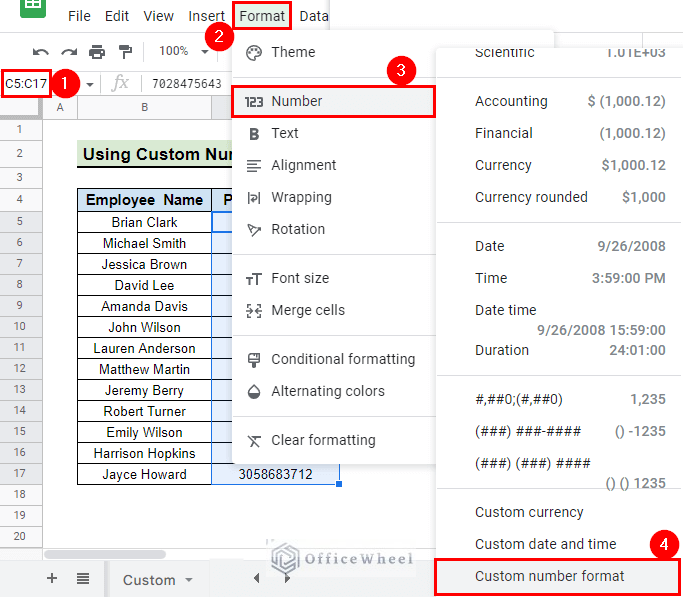
- Next, you will see a Custom number formats dialogue box appear.
- Type the following custom number format in the dialogue box and click on Apply to apply the custom format to the selected cells.
(###) ###-####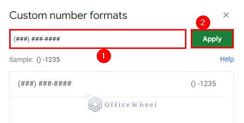
The parentheses around the first three digits indicate the area code of the phone number.
- Finally, you have applied the custom format to the selected cells.
II. Utilizing REGEXREPLACE Function
The REGEXREPLACE function can be used with the TEXT function to customize phone numbers with parentheses. We use the same dataset we used in the previous method.
Steps:
- First, go to the cell where you want to apply the formula. We go to cell D5 in our example.
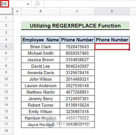
- Then, type the following formula:
=TEXT(REGEXREPLACE(TEXT(C5,"@"),"\D+",""),"(###) ###-####")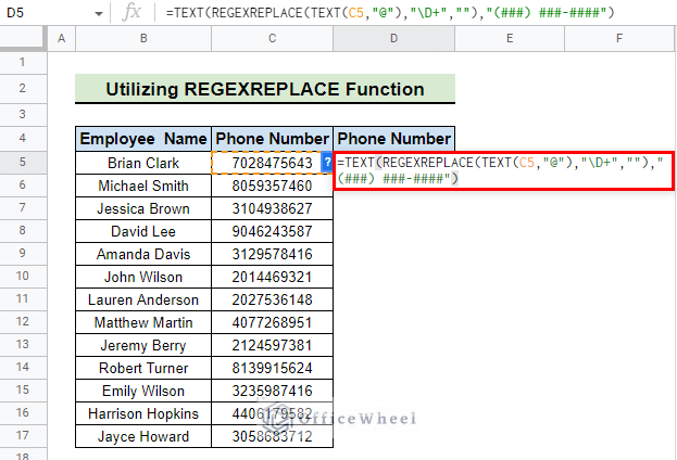
Formula Explanation:
TEXT(C5,”@”)
- The TEXT function formats the contents of cell C5 as text and replaces the decimal point with the @ symbol.
REGEXREPLACE(TEXT(C5,”@”),”\D+”,””)
- “\D+” matches one or more non-numeric characters.
- “” indicates replacing all matches with an empty string.
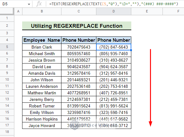
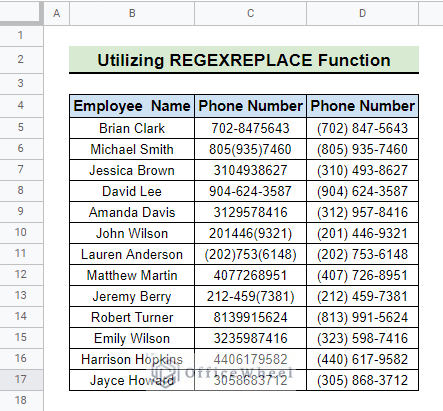
TEXT(REGEXREPLACE(TEXT(C5,”@”),”\D+”,””),”(###) ###-####”)
- The TEXT function formats the result of REGEXREPLACE as a phone number in the format (###) ###-####.
- Finally, press ENTER to display the phone numbers according to the format. Use autofill to copy the formula to the cells below.
Read More: How to Insert Serial Numbers in Google Sheets (7 Easy Ways)
4. Apply Parentheses Around Any Number by Taking Advantage of Regular Expressions
The REGEXREPLACE function in Google Sheets offers a convenient solution for modifying text in your spreadsheets. With this function, you can add brackets to numbers in your sheet with ease.
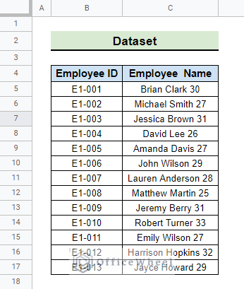
We have a dataset with some Employee ID and Employee Name with their Age in it. The Employee Name and Age are in a single column. We will use this dataset to apply parentheses around the age.
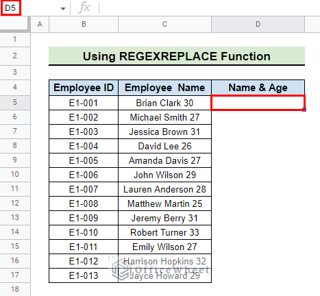
- First, go to the cell where you want to add brackets around the numbers. We go to cell D5 for our example.
- After that, type the following formula:
=REGEXREPLACE(C5, "(\d+)", "($1)")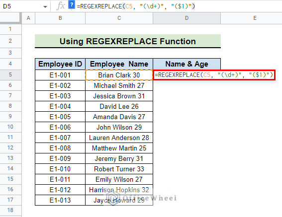
Formula Explanation:
REGEXREPLACE(C5, “(\d+)”, “($1)”)
- C5 is the cell reference that contains the text to modify.
- (\d+) matches any digit (0-9), and the + symbol means one or more.
- “($1)” is the replacement string, where $1 refers to the sequence of digits matched by (\d+). The brackets enclose the numbers matched by the regular expression.
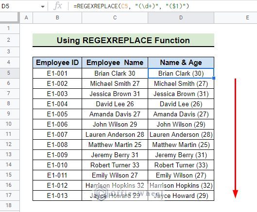
- Finally, press ENTER to display the numbers wrapped in parentheses. Use autofill to copy the formula to the cells below.
Implementing Numbers Wrapped in Parentheses for QUERY Function Select Clause
The QUERY function in Google Sheets allows us to perform SQL-like queries on data ranges. In the previous method, we have shown you how we can use the REGEXREPLACE function to add parentheses around numbers. We will employ the above REGEXREPLACE formula to dynamically reference columns with the QUERY function Select clause.
We will sum columns C, D, E, and F (the 2nd, 3rd, 4th, and 5th columns in range B4:F) in our dataset by using the SUM aggregation function within the QUERY function.
=QUERY({B4:F},"Select SUM(Col2),SUM(Col3),SUM(Col4),SUM(Col5)",1)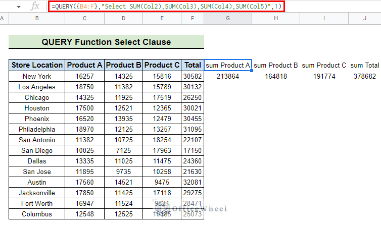
If we add a column before column F, the dataset will adjust automatically.
To resolve that, we will utilize the REGEXREPLACE formula, as employed in the previous method, to make the QUERY function dynamic.
Steps:
- The QUERY syntax that is not dynamic is:
"Select SUM(Col2),SUM(Col3),SUM(Col4),SUM(Col5)"- The SEQUENCE function can dynamically generate the columns to sum.
=SEQUENCE(1,COLUMNS(C4:F4),2)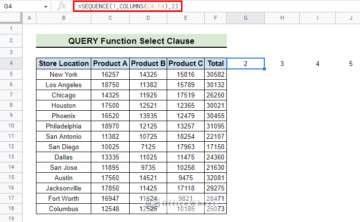
- The SEQUENCE formula adjusts automatically for any new columns in the range C4:F4.
- The REGEXREPLACE formula syntax that we used in the previous method that adds parentheses around numbers is as follows:
REGEXREPLACE(text, "(\d+)", "($1)")- We have to replace the text argument with the SEQUENCE formula. However, the output of the SEQUENCE function is a number with multiple columns, and as a result, it won’t work. To resolve this, we need to add the argument &”” at the end of the SEQUENCE function.
=REGEXREPLACE(SEQUENCE(1,COLUMNS(C1:F1),2)&"","(\D+)", "($1)")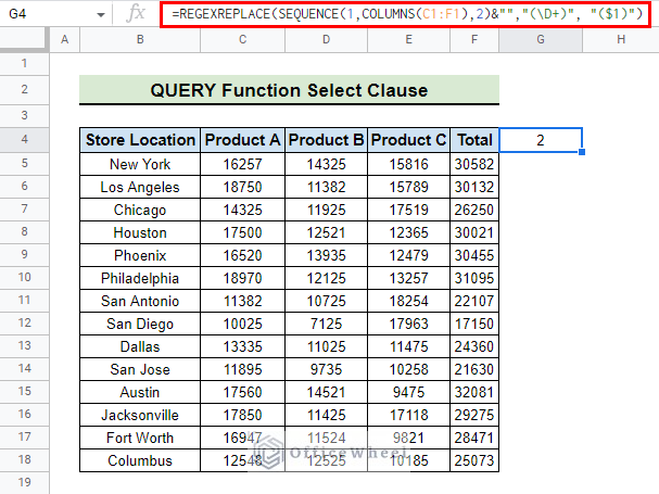
- We need to enclose the formula with the ARRAYFORMULA function as the text argument in the REGEXREPLACE function is an array.
=ARRAYFORMULA(REGEXREPLACE(SEQUENCE(1,COLUMNS(C4:F4),2)&"","(\D+)", "($1)"))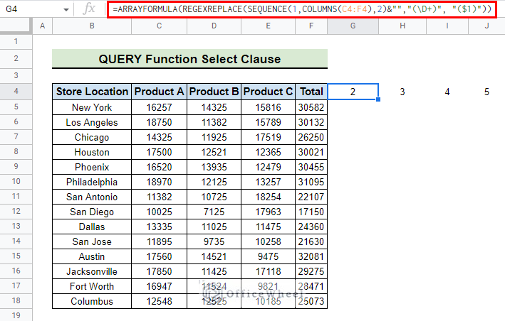
- We modify the formula to get Sum of the columns:
=ARRAYFORMULA(REGEXREPLACE(SEQUENCE(1,COLUMNS(C4:F4),2)&"","(\d+)", "SUM(Col$1)"))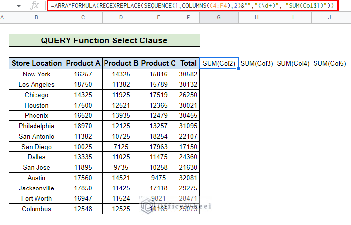
- Then, we use the TEXTJOIN function to join these outputs in a single column.
=TEXTJOIN(",",TRUE,ARRAYFORMULA(REGEXREPLACE(sequence(1,columns(C4:F4),2)&"","(\d+)", "Sum(Col$1)")))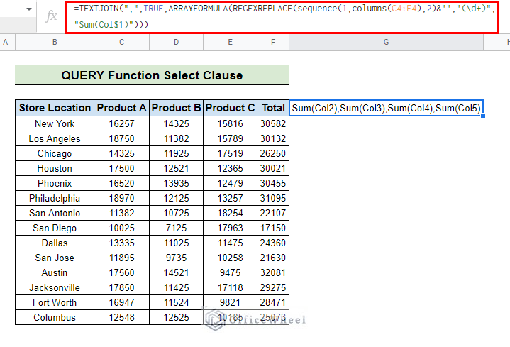
- Finally, this is what the QUERY formula looks like:
=QUERY({B4:F},"Select "&TEXTJOIN(",",TRUE,ARRAYFORMULA(REGEXREPLACE(SEQUENCE(1,COLUMNS(C4:F4),2)&"","(\d+)", "SUM(Col$1)"))),1)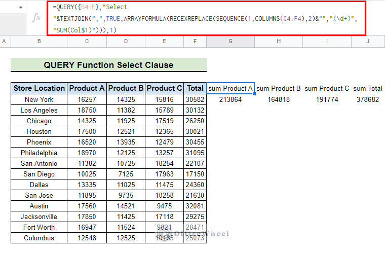
Read More: How to Make a Tournament Bracket in Google Sheets (Easy Steps)
5. Add Vertical Parentheses
The vertical parentheses allow you to create custom functions and calculations to make it easier to automate tasks and perform more complex computations in your spreadsheets.
But, Google Sheets does not allow us to add vertical parentheses directly from there. So we have to bypass this problem to add vertical parentheses in Google Sheets.
Steps:
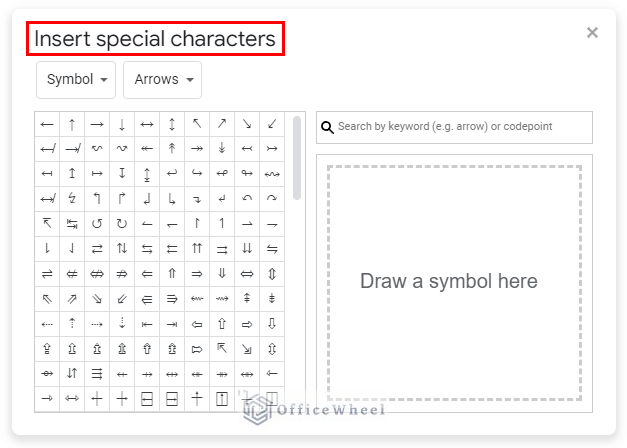
- First, open a Google Docs document and go to Menu bar > Insert > Special characters.
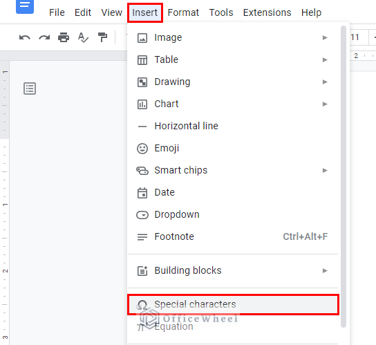
- After that, you will see a window appear named Insert special characters.
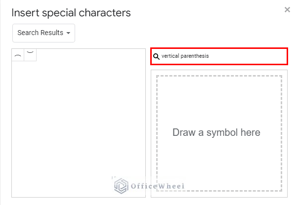
- Then, in the search box, type vertical parenthesis to look for the vertical parentheses.
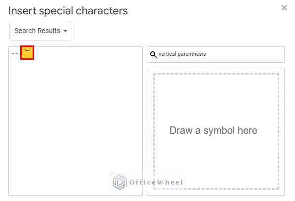
- After that, click on the characters to add them to the doc.
- Then, you can select and copy these using the mouse or the keyboard shortcut CTRL+C. The vertical parentheses have now been copied to the clipboard.
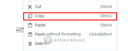
- Finally, you can add these to your Google Sheets documents whenever necessary.
Conclusion
This article explains the ways to add parentheses in Google Sheets. We recommend you try out the methods in order to have a better understanding of the methods. The intention of this article is to offer useful information and assist you in achieving your goal.
Additionally, consider looking into other articles available on OfficeWheel to expand your understanding and skill in using Google Sheets.
Related Articles
- How to Insert Superscript in Google Sheets (2 Simple Ways)
- Insert Button in Google Sheets (5 Quick Steps)
- How to Insert Error Bars in Google Sheets (3 Practical Examples)
- Insert Blank Column Using QUERY in Google Sheets
- How to Insert Yes or No Box in Google Sheets (2 Easy Ways)
- Insert a Drop-Down List in Google Sheets (2 Easy Ways)
- How to Insert Sparklines in Google Sheets (4 Useful Examples)