Use of Google Sheets INDEX MATCH in Multiple Columns

In Google Sheets, the INDEX MATCH function is the combination of two basic functions: INDEX and MATCH function. Though separately these two functions act like basic ones, together they are more powerful and effective. They can even be used as an alternative to the VLOOKUP function. In this article, we will learn step by step the use of Google Sheets INDEX MATCH in multiple columns.

Table of Contents

A Sample of Practice Spreadsheet

You can download spreadsheets from here and practice.

Use of INDEX MATCH with Multiple Columns

Steps to Use INDEX MATCH with Multiple Columns in Google Sheets

When you use the INDEX MATCH function, you have to start with the INDEX function first. The MATCH function will place the argument within the INDEX function. To apply this function for multiple columns you can apply the following syntax:

=INDEX(reference,MATCH(1,(criteria1)*(criteria2)*(criteria3),0))

Here, reference represents the range from where we will get the result, MATCH provides the position of the search key, 1 is used as a fixed search key, criteria1, criteria2,criteria3…. is the condition to match, 0 is set to return the exact value.

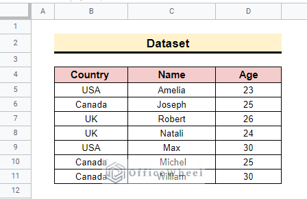
Step 1: Create a Dataset

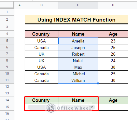
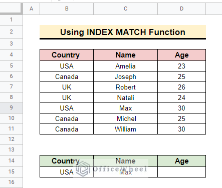
To apply the INDEX MATCH formula for multiple columns you have to develop a dataset that contains some interrelated columns. Here, we develop a dataset that represents some respondent information. The dataset contains three columns: Country, Name and Age.

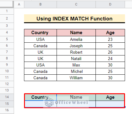
We also create a table containing the same column name to show the final result.

Step 2: Insert Search Keys

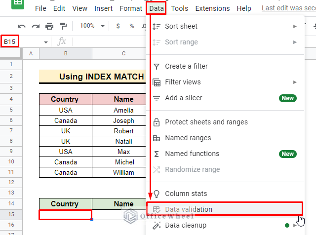
For inserting the search key first, you can create a dropdown list which will help you to find your values easily. As it is an optional method, you can directly insert your search key in the newly developed table. Here, we create a dropdown list. So, for inserting the search key,

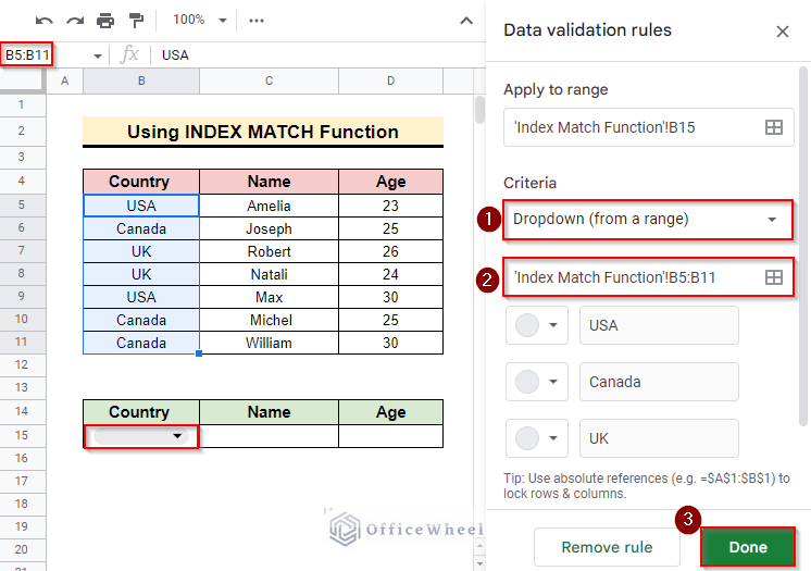
First, select cell B15 where we want to input the search key. Then go to Data and select the Data validation option.

After that, select Dropdown (from a range), then specify the range B5:B11. Finally, press OK to add the dropdown in the cell.

In the same way, insert a dropdown list for other columns.

When you click on the dropdown symbol you can find all the values of the specific column. You can now insert any of them as a search key.

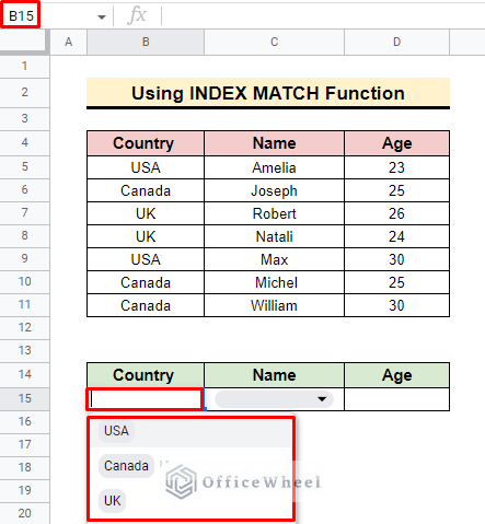
So, insert the search key for multiple columns.

You can also insert them directly from the dataset.

Similar Readings

Step 3: Apply INDEX MATCH Function

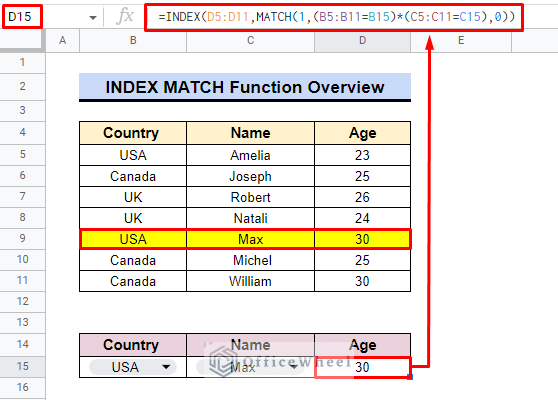
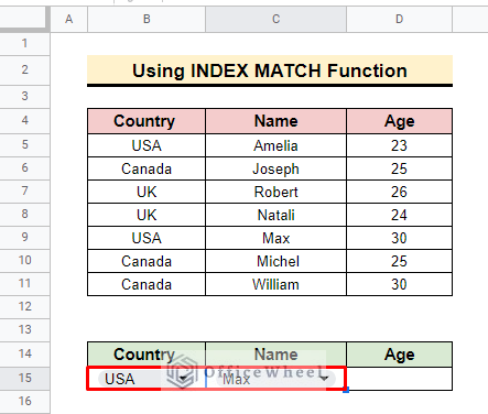
After selecting search keys for the function now apply the INDEX MATCH function for multiple columns. Here, we insert search keys ‘USA’ and ‘Max’. Now, to look up the age of these search keys,

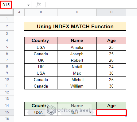
First, select cell D15 to apply the INDEX MATCH formula.

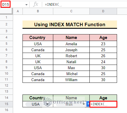
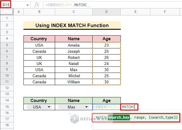
At the beginning insert the INDEX function.

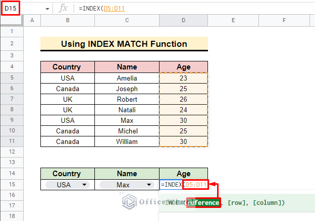
As reference insert the range D5:D11 which represents the Age column of the source dataset.

After that insert the MATCH function.

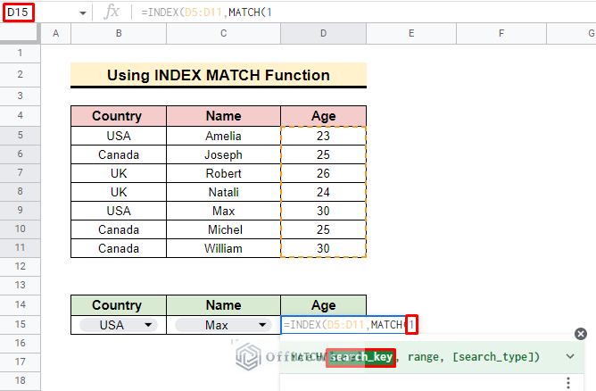
Now, add 1 as a fixed search key.

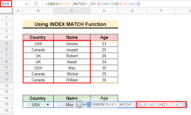
Then input the criteria or conditions for multiple columns. Here we add B5:B11=B15 and C5:C11=C15. Connect these statements with multiple symbol “*”.

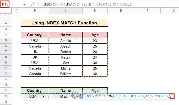
In the end, input 0 to get the exact value for the formula.

Step 4: Final Output

To get the final output press ENTER and you will find the desired value in your selected cell.

=INDEX(D5:D11,MATCH(B5:B11=B15)*(C5:C11=C15),0))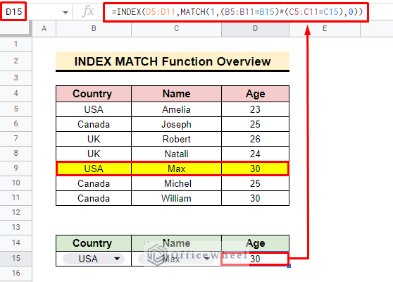

In this way, you can get any value from any dataset whether it is large or small in size.

Things to Remember

You have to apply the INDEX function first.
Insert the range carefully.
Always use “*” while inserting criteria.

Conclusion

We believe that after completing the article, you have built a clear knowledge of Google Sheets INDEX MATCH multiple columns. To explore more about Google Sheets, you can visit the OfficeWheel website.