When utilizing the VLOOKUP function, the search column must be the first column from the left in your lookup table for it to operate. This limits your search options to the left to the right exclusively. However, you may search to the left in your lookup table. In this article, I will show 4 simple examples of VLOOKUP to the left in Google Sheets.
4 Simple Ways to VLOOKUP Left in Google Sheets
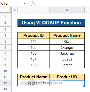
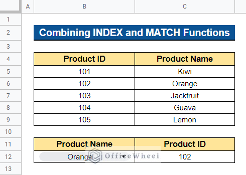
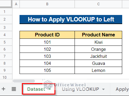
We will use the dataset below to demonstrate the examples of VLOOKUP to the left in Google Sheets. The dataset contains the Product ID and Product Name of a shop. Now, using the search column for Product Name, we want to look for the value of Product ID.

1. Using VLOOKUP Function
We can use an array to build a new virtual table with the columns reversed so that we can do a VLOOKUP on this short-term virtual table and perform the operation to the left. Remember that the column being reversed does not have to be continuous.
Steps:
- First, select a cell where you want to apply the formula. We want to know the Product ID in Cell C12 based on the Product Name in Cell B12. So, we selected Cell C12.
- Now, type the formula below and press Enter–
=VLOOKUP(B12,{C5:C9,B5:B9},2,FALSE)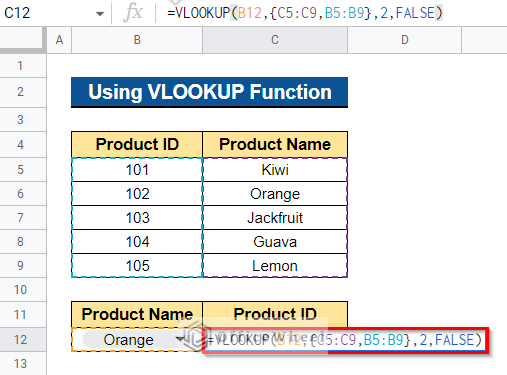
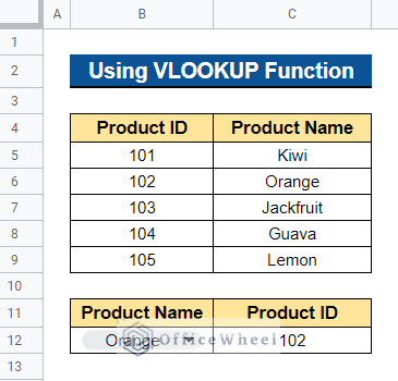
- Thus, it will show the Product ID based on the Product Name in Cell B12.
Read More: Alternative to Use VLOOKUP Function in Google Sheets
2. Applying XLOOKUP Function
The XLOOKUP function is the most effective VLOOKUP substitute. You may search for a value in any row or column using the XLOOKUP function, and it will return the value of a cell in a separate row or column that matches your search word. We can find exact matches and can look up in any direction using the XLOOKUP function.
Steps:
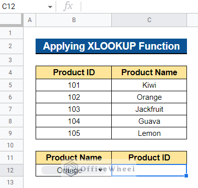
- Choose a cell to which you will first apply the formula. Using the Product Name in Cell B12 as our basis, we wish to know the Product ID in Cell C12. So we chose Cell C12.
- Press the Enter button after typing the formula below-
=XLOOKUP(B12,C5:C9,B5:B9)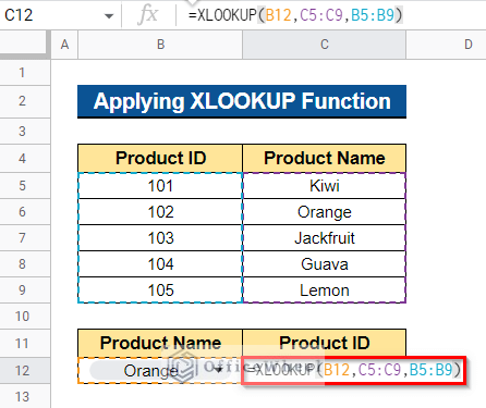
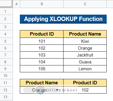
- As a result, it will display the Product ID based on the Product Name in Cell B12.
Read More: How to VLOOKUP Last Match in Google Sheets (5 Simple Ways)
3. Combining INDEX and MATCH Functions
The VLOOKUP function may not work properly if the lookup column is not the first column in the lookup table. In these circumstances, we may search for values to the left by using the combination of the INDEX and MATCH functions. One benefit of this approach is that the value won’t change if we add or remove columns from the lookup table.
Steps:
- First, choose the cell to which you wish to apply the formula. Based on the Product Name in Cell B12, we want to know the Product ID in Cell C12. So, we chose Cell C12.
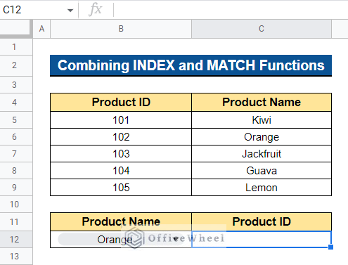
- To continue, enter the formula below and hit Enter–
=INDEX(B5:B9,MATCH(B12,C5:C9,0))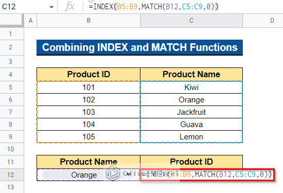
Formula Breakdown
- MATCH(B12,C5:C9,0)
First, the MATCH function returns the position of Cell B12 in a range of Cell C5:C9 that matches a given value relative to other items in the range.
- INDEX(B5:B9,MATCH(B12,C5:C9,0))
Then the INDEX function will give back the content of a cell, defined by the column and row offset.
- As a result, depending on the Product Name in Cell B12, the Product ID will be shown.
Read More: Combine VLOOKUP and HLOOKUP Functions in Google Sheets
Similar Readings
- Google Sheets HLOOKUP to Return Column (3 Simple Ways)
- How to Create Conditional Drop Down List in Google Sheets
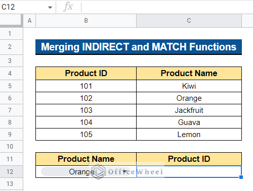
4. Merging INDIRECT and MATCH Functions
We can also use the combination of the INDIRECT and MATCH functions to look up a value to the left in Google Sheets.
Steps:
- First, select the cell to which you wish to apply the formula. In our case, we selected Cell C12.
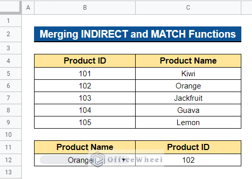
- Now, type the following formula and hit the Enter key-
=INDIRECT("B"&MATCH(B12,C5:C9,0)+4)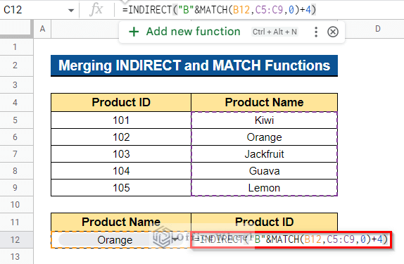
Formula Breakdown
- MATCH(B12,C5:C9,0)
The MATCH function initially returns Cell B12‘s location in a range of Cell C5:C9 that corresponds to a specified value in relation to other items in the range.
- INDIRECT(“B”&MATCH(B12,C5:C9,0)+4)
Then the INDIRECT function gives back the cell reference defined by the string.
- Thus, you will get the desired output.
How to Do Reverse VLOOKUP from Another Sheet in Google Sheets?
We frequently need to pull data from one sheet while working on another. To retrieve VLOOKUP to the left from another sheet, you can use any of the four ways that were just covered. We’ll apply the XLOOKUP function in this case.
Steps:
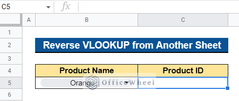
- We want to exact data from the worksheet named Dataset.
- To do this, first select a cell to which you want to apply the formula. Based on the Product Name in Cell B5, we want to know the Product ID in Cell C5. So, we selected Cell C5.
- Now, enter the formula below and hit Enter–
=XLOOKUP(B5,Dataset!C5:C9,Dataset!B5:B9)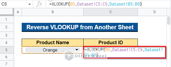
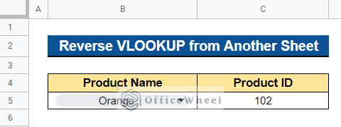
- Thus, you will get the Product ID based on the Product Name in Cell B5.
Read More: Google Sheets Vlookup Dynamic Range
Conclusion
In this article, I have shown 4 simple examples to apply the VLOOKUP function to the left in Google Sheets. I have also shown how to do reverse VLOOKUP from another sheet in Google Sheets. Please feel free to ask any questions or suggest any ideas. Visit Officewheel.com to explore more.
Related Articles
- [Fixed!] INDEX MATCH Is Not Working in Google Sheets (5 Fixes)
- Google Sheets Conditional Formatting with INDEX-MATCH
- Use of Google Sheets INDEX MATCH in Multiple Columns
- Find All Cells With Value in Google Sheets (An Easy Guide)
- Match Multiple Values in Google Sheets (An Easy Guide)
- VLOOKUP Error in Google Sheets (with Quick Solutions)
- VLOOKUP with IMPORTRANGE Function in Google Sheets
- How to Use VLOOKUP with IF Statement in Google Sheets