The VLOOKUP function is a very dynamic tool in Google Sheets. It’s one of the most used functions in Google Sheets. We can use this function to look for any value vertically in any given range of data. In this article, I’ll show you 8 suitable examples of how to use the VLOOKUP function in Google Sheets with clear images and steps.
What Is VLOOKUP Function in Google Sheets?
The VLOOKUP function in Google Sheets searches for any information by row.
Syntax
The syntax of the VLOOKUP function is like this below-
=VLOOKUP(search_key, range, index, [is_sorted])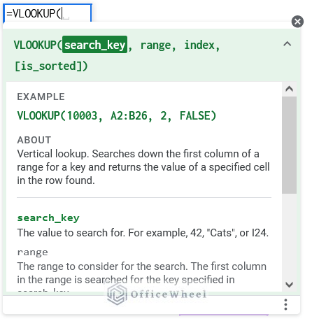
Arguments
| Argument | Requirement | Function |
|---|---|---|
| Search key | Required | Reference or value to search for |
| Range | Required | Reference where to search for |
| Index | Required | The column no of the return value |
| Is sorted | Optional | Data is sorted or not (FALSE for the exact match and TRUE for the approximate match) |
Output
The formula VLOOKUP(10003,A2:B6,2,FALSE) will search for the value 10003 in the range Cell A2 to B6 and returns an exact value from Column No 2.
8 Suitable Examples to Use the VLOOKUP Function in Google Sheets
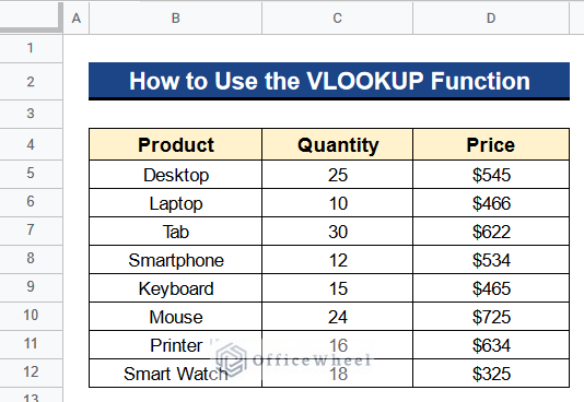
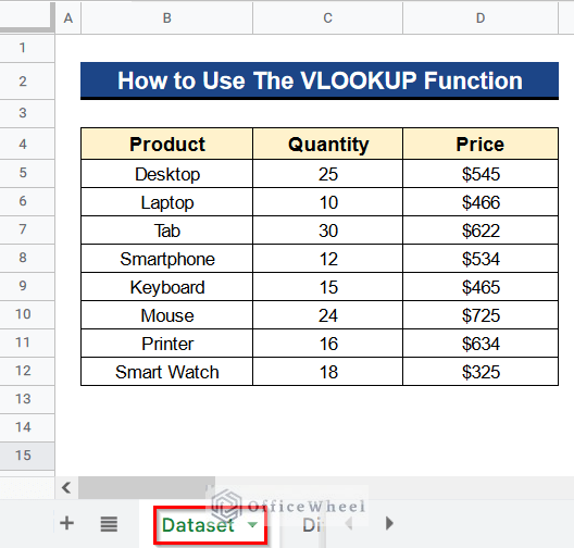
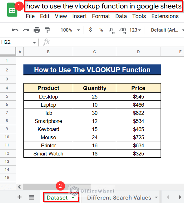
Let’s get introduced to our dataset first. Here we have some products in Column B, their quantities in Column C, and their prices in Column D. We’ll now see 8 useful examples of how to use the VLOOKUP function in Google Sheets with the help of this dataset.
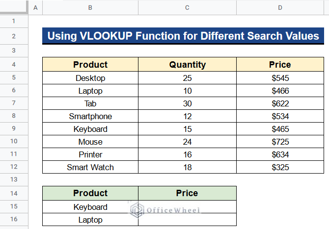
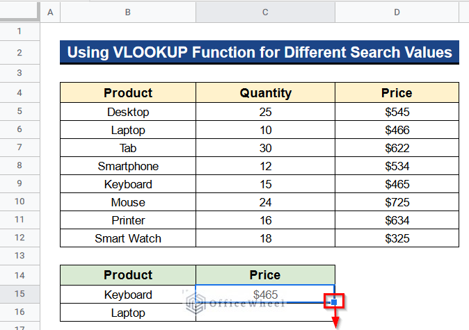
Example 1: Using VLOOKUP Function for Different Search Values
Firstly, we’ll use the VLOOKUP function for searching different values. We have 2 values in our dataset as you can see below. We’ll search for them in our dataset.
Steps:
- At first, type the following formula in Cell C15–
=VLOOKUP(B15,$B$5:$D$12,3,FALSE)- Then, hit Enter to get the corresponding price.
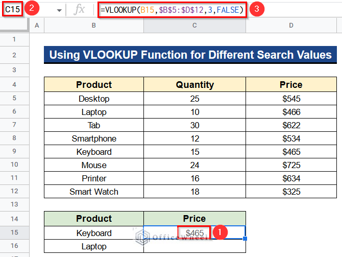
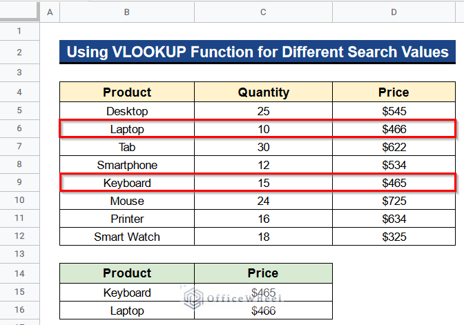
- Finally, you’ll see that the results are matching with the dataset.
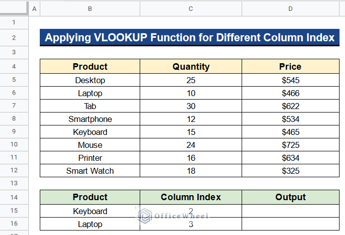
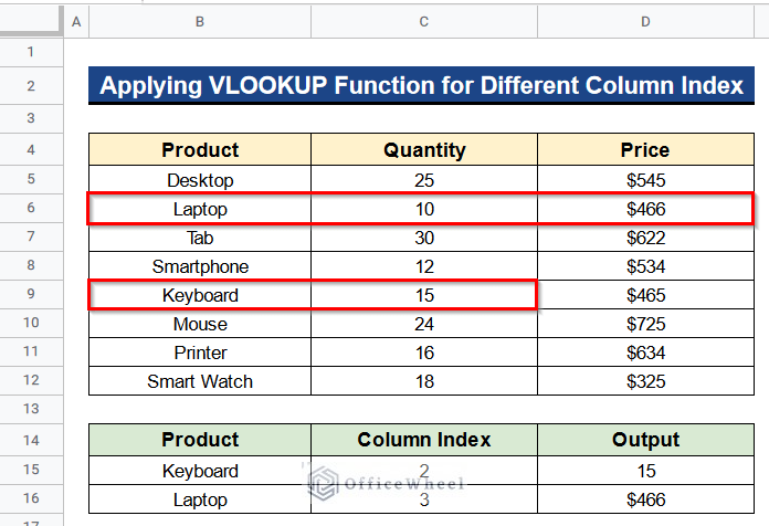
Example 2: Applying VLOOKUP Function for Different Column Index
Now we have put different column index numbers beside our search values and so it will return values from different columns. You’ll find this in the attached picture. And we want to search for the values based on them. Let’s see the steps of how to use the VLOOKUP function in Google Sheets.
Steps:
- First of all, write the following formula in Cell D15–
=VLOOKUP(B15,$B$5:$D$12,C15,FALSE)- After that, press Enter to get the output.
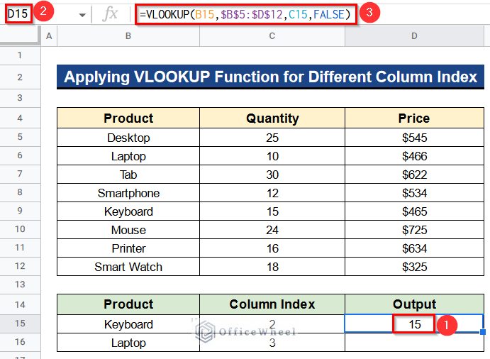
- Thereafter, use the Fill Handle tool for the rest of the cells.
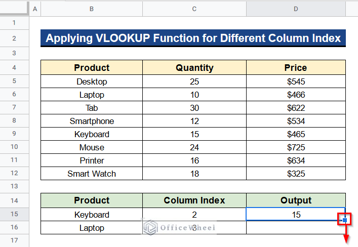
- At last, you’ll find that the results are different because we have put different column index numbers.
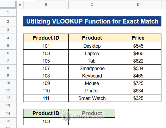
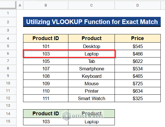
Example 3: Utilizing VLOOKUP Function for Exact Match
Now we have a slightly different dataset. We have product ids in Column B, products in Column C, and their prices in Column D. We want to exactly match the product id in the below picture with our dataset and want to get the corresponding product. So we’ll insert FALSE into the VLOOKUP function to exactly match the value.
Steps:
- In the first instance, put the following formula in Cell C15–
=VLOOKUP(B15,$B$5:$D$12,2,FALSE)- Thereafter, click Enter to get the product.
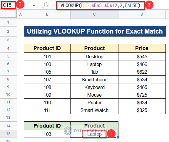
- Ultimately, the exact result will be the output.
Read More: How to Use VLOOKUP Function for Exact Match in Google Sheets
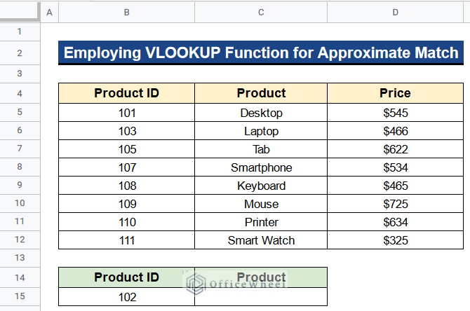
Example 4: Employing VLOOKUP Function for Approximate Match
We have to match a product id, 102 which is not present in our dataset. Therefore we’ll insert TRUE into the VLOOKUP function to approximately match the value.
Steps:
- In the first place, insert the following formula in Cell C15–
=VLOOKUP(B15,$B$5:$D$12,2,TRUE)- Afterward, hit the Enter Button to get the product.
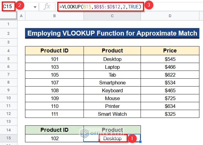
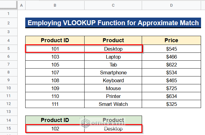
- In the end, notice that our product id is 102. But it is giving the result for product id 101. So we are getting an approximate result.
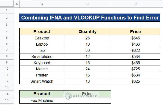
Example 5: Combining IFNA and VLOOKUP Functions to Find Error
If we search for a product that is absent in our dataset, then using the VLOOKUP function will give an error message. But we want to get our output as “Not Found”. We can do this by combining the IFNA and VLOOKUP functions. So we’ll search for the product Fax Machine which is not present in the dataset and bring out the result as “Not Found”.
Steps:
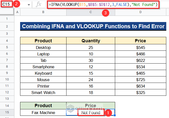
- In the beginning, type the following formula in Cell C15–
=IFNA(VLOOKUP(B15,$B$5:$D$12,3,FALSE),"Not Found")- Consequently, press the Enter Button to get the result.
Formula Breakdown
- VLOOKUP(B15,$B$5:$D$12,3,FALSE)
First, this function will look for the value in Cell B15 from the range Cell B5 to D12 and give the price.
- IFNA(VLOOKUP(B15,$B$5:$D$12,3,FALSE),”Not Found”)
Then this function will give “Not Found” as output because the VLOOKUP function is not finding the value in the dataset.
Read More: VLOOKUP Error in Google Sheets (with Quick Solutions)
Similar Readings
- How to Do Reverse VLOOKUP in Google Sheets (4 Useful Ways)
- Google Sheets Vlookup Dynamic Range
- How to VLOOKUP for Partial Match in Google Sheets
- [Fixed!] Google Sheets If VLOOKUP Not Found (3 Suitable Solutions)
- How to VLOOKUP Between Two Google Sheets (2 Ideal Examples)
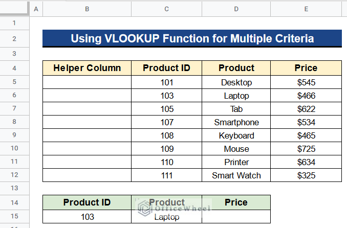
Example 6: Using VLOOKUP Function for Multiple Criteria
Look at a different problem now. We have both the product id and product. And we want to get results for these multiple criteria using the VLOOKUP function. For this purpose, we need to create a helper column first. Then we have to unite the VLOOKUP and JOIN functions together. Let’s see how to do it.
Steps:
- Before all, write the following formula in Cell B5–
=JOIN(" ",C5:D5)- Again, click the Enter Button to get the output.
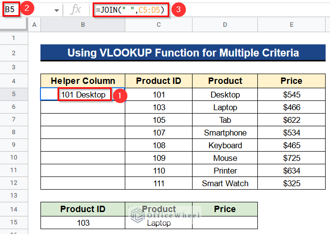
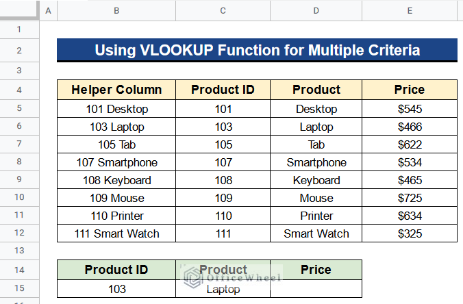
- Moreover, apply the Fill Handle tool to get results for Column B.
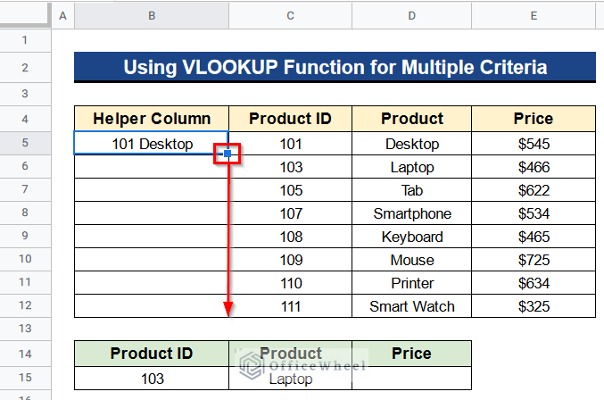
- Then, you’ll get that the product ids and products are in a combo in Column B.
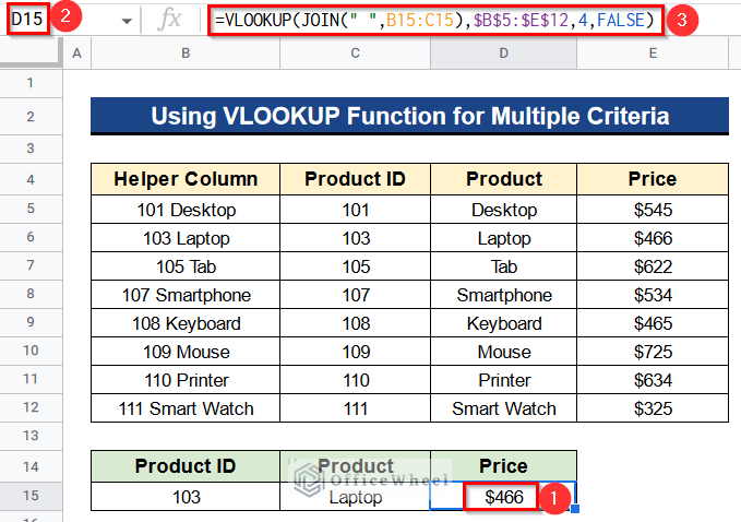
- Next, insert the following formula in Cell D15–
=VLOOKUP(JOIN(" ",B15:C15),$B$5:$E$12,4,FALSE)- After that, hit Enter to get the price.
Formula Breakdown
- JOIN(” “,B15:C15)
Foremost, this function will join the values of Cell B15 and C15.
- VLOOKUP(JOIN(” “,B15:C15),$B$5:$E$12,4,FALSE)
Next, this function will look for the joined values in our dataset and gives the result.
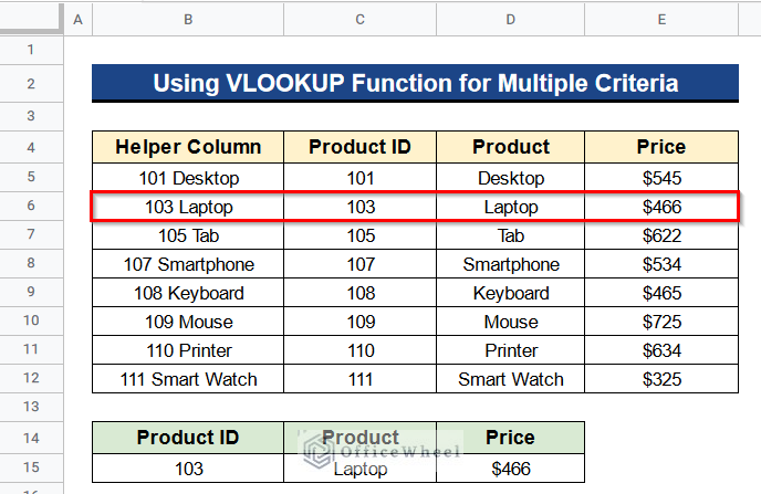
- Finally, we are getting results for both criteria, product id, and product.
Read more: How to VLOOKUP with Multiple Criteria in Google Sheets
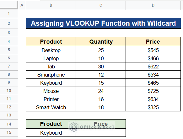
Example 7: Assigning VLOOKUP Function with Wildcard
We can further use the VLOOKUP function with Wildcard to get results for partial matching. We’ll use the Asterisk Wildcard (*) with the function to get results for the character “Key” in our case. These characters will match with the product Keyboard and give its price.
Steps:
- Earlier on, put the following formula in Cell C15–
=VLOOKUP("Key*",B5:D12,3,FALSE)- Then, press Enter to get the result.
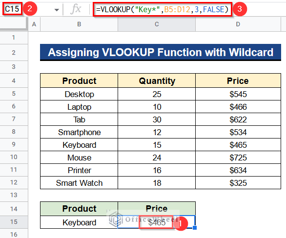
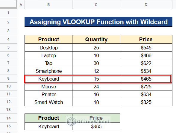
- At last, you’ll see that it is matching with the dataset and giving the actual result.
Read More: How to Use VLOOKUP Function with Wildcard in Google Sheets
Example 8: Applying VLOOKUP Function on Another Sheet
Consequently, we can apply the VLOOKUP function in another Google Sheet. I’ll show 2 processes regarding this.
8.1: Another Sheet in Same File
We can use the VLOOKUP function in another sheet of the same Google Sheet.
Steps:
- Before, rename the original sheet as Dataset.
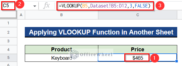
- Next, move to a new sheet and write the following formula in Cell C5–
=VLOOKUP(B5,Dataset!B5:D12,3,FALSE)- After that, click Enter to get the result instantly.
Read More: How to Use VLOOKUP to Import from Another Workbook in Google Sheets
8.2: Another Sheet in Different File
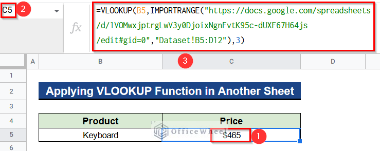
Additionally, we can also use the VLOOKUP function in another sheet of a different Google Sheet. For this purpose, we’ll combine the VLOOKUP function with the IMPORTRANGE function.
Steps:
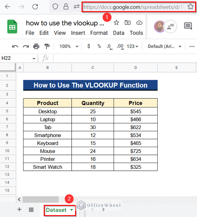
- Initially, give a name to our original Google Sheet. Here we have given the name “how to use the vlookup function in google sheets”.
- Moreover, give a name of the sheet also. Here we have given the name “Dataset”.
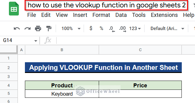
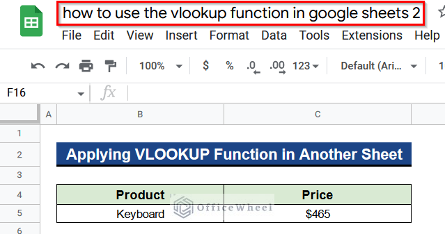
- Then go to an entirely new Google Sheets and give it a different name. Like we have given it the name “how to use the vlookup function in google sheets 2”.
- We’ll now look for the product Keyboard from our original Google Sheets.
- So copy the link from the original Google Sheet.
- Then, insert the following formula in Cell C5–
=VLOOKUP(B5,IMPORTRANGE("https://docs.google.com/spreadsheets/d/1VOMwxjptrgLwV3y0DjoixNgnFvtK95c-dUXF67H64js/edit#gid=0","Dataset!B5:D12"),3)- Afterward, hit the Enter Button to get the result quickly.
Formula Breakdown
- IMPORTRANGE(“https://docs.google.com/spreadsheets/d/1VOMwxjptrgLwV3y0DjoixNgnFvtK95c-dUXF67H64js/edit#gid=0″,”Dataset!B5:D12”)
Foremost, this function will import data from the previous Google Sheets.
- VLOOKUP(B5,IMPORTRANGE(“https://docs.google.com/spreadsheets/d/1VOMwxjptrgLwV3y0DjoixNgnFvtK95c-dUXF67H64js/edit#gid=0″,”Dataset!B5:D12”),3)
Next, this function will look for the values of Cell B5 in the imported data and give results.
- In the end, you can notice that the VLOOKUP function is working fine in the new Google Sheets.
Read More: Alternative to Use VLOOKUP Function in Google Sheets
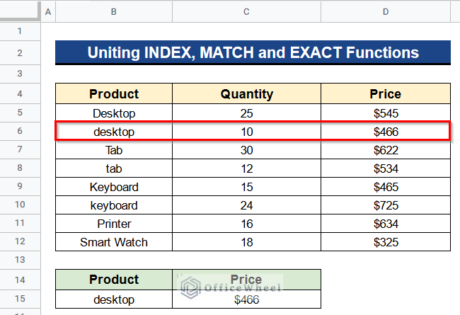
How to Unite INDEX, MATCH and EXACT Functions for Case Sensitive Values Instead of VLOOKUP Function in Google Sheets
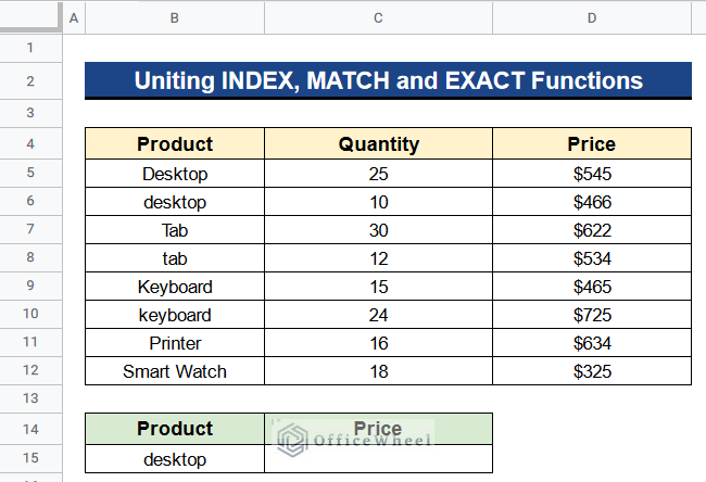
The VLOOKUP function is case insensitive. So if we have such data which has case-sensitive values then using the VLOOKUP function will give erroneous results. To solve this issue we can use the combination of the INDEX, MATCH, and EXACT functions. Now we have a case-sensitive value which is “desktop” and we’ll look for it in our dataset by using these functions.
Steps:
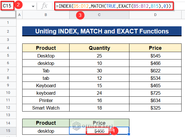
- Firstly, type the following formula in Cell C15–
=INDEX(D5:D12,MATCH(TRUE,EXACT(B5:B12,B15),0))- Consequently, press the Enter Button to get the price.
Formula Breakdown
- EXACT(B5:B12,B15)
At first, this function tests for the identical value in Cell B15 in the range Cell B5 to B12.
- MATCH(TRUE,EXACT(B5:B12,B15),0)
Next, this function gives the relative position of the identical value.
- INDEX(D5:D12,MATCH(TRUE,EXACT(B5:B12,B15),0))
Lastly, this function gives the result based on matching values.
- Finally, you’ll see that the small case letters are matching with the small case and giving correct results.
Read More: How to VLOOKUP All Matches in Google Sheets (2 Approaches)
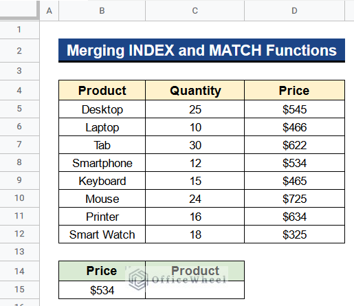
How to Merge INDEX and MATCH Functions Instead of VLOOKUP Function to Search on Left Side in Google Sheets
The VLOOKUP function has a limitation. It can only look for a value on the right side and the lookup value must be in the first column of the range. But what if we want to search on the left side of the data? There is a very easy solution to that. We can merge the INDEX and MATCH functions to search on the left side. Like now we want the names of the products based on price. Let’s see the steps.
Steps:
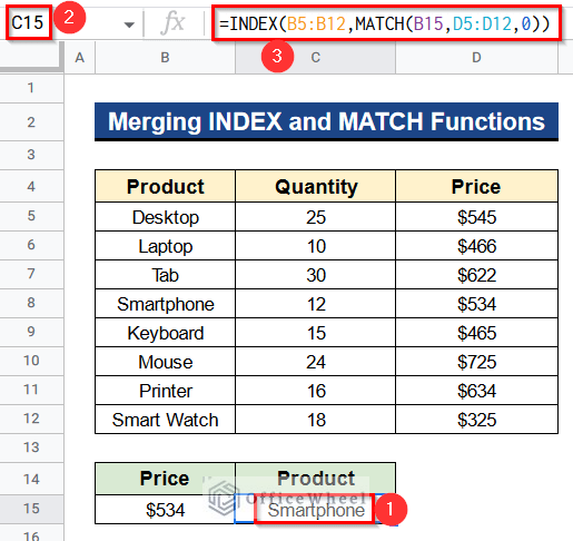
- First, write the following formula in Cell C15–
=INDEX(B5:B12,MATCH(B15,D5:D12,0))- Again, click the Enter Button to get the product.
Formula Breakdown
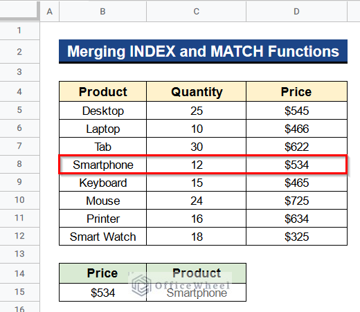
- MATCH(B15,D5:D12,0)
Before, this function returns the relative position of the value in Cell B15 from the range Cell D5 to D12.
- INDEX(B5:B12,MATCH(B15,D5:D12,0))
Then this function gives the output from Cell B5 to B12 based on the former match.
- Ultimately, you’ll get the exact match.
Conclusion
That’s all for now. Thank you for reading this article. In this article, I have discussed 8 suitable examples of how to use the VLOOKUP function in Google Sheets. I have also discussed what to do if there is case-sensitive value. In addition to that, I have talked about the process if you want to search for any value on the left side of the dataset. Please comment in the comment section if you have any queries about this article. You will also find different articles related to google sheets on our officewheel.com. Visit the site and explore more.
Related Articles
- How to VLOOKUP Left in Google Sheets (4 Simple Ways)
- Use IFERROR with VLOOKUP Function in Google Sheets
- How to Use VLOOKUP for Conditional Formatting in Google Sheets
- VLOOKUP Last Match in Google Sheets (5 Simple Ways)
- How to Concatenate with VLOOKUP in Google Sheets
- Use Wildcard in Google Sheets (3 Practical Examples)
- How to Use VLOOKUP with Drop Down List in Google Sheets