Named range can be a useful feature in Google Sheets if you are working with a large volume of data. It can help you memorize important parts of your range or a full range by naming them with unique names. In this article, we will discuss how you can use VLOOKUP with a named range in Google Sheets easily and effectively.
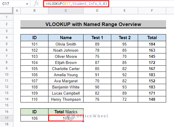
The above screenshot is an overview of the article, representing how we can use VLOOKUP with named range in Google Sheets.
A Sample of Practice Spreadsheet
Download this spreadsheet to practice yourself.
What Is Named Range in Google Sheets?
A Named Range allows you to give a unique name to important parts of a range or a full range in Google Sheets. The ability to use Named Range in functions and formulas can help you manage your data easily and help you save precious time.
We have a data table with employee Names and their respective Sales Amount, we named the Sales Amount range which is C5:C9 as Sales.
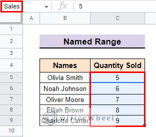
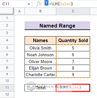
We use this named range to calculate the Total sales made by the employees.
How to Apply Named Range in Google Sheets
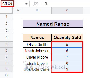
Consider the dataset we used before. The table contains employee Names and their respective Sales Amount. We will try to name the Sales Amount range with Named Range.
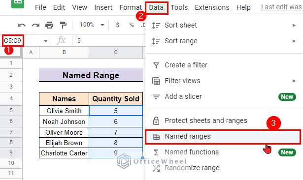
- First, select the range where you want to apply the Named Range. We select Range C5:C9 in our example.
- Then, go to Menu bar > Data > Named ranges.
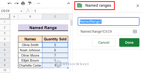
- Now, you will see a sidebar called Named ranges appear on the right side of your workbook.
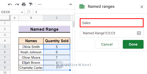
- After that, input the name that you want to use for your selected range. We use Sales as the name in our example.
- Then, you can even select a different range from the Select data range icon on the side panel.
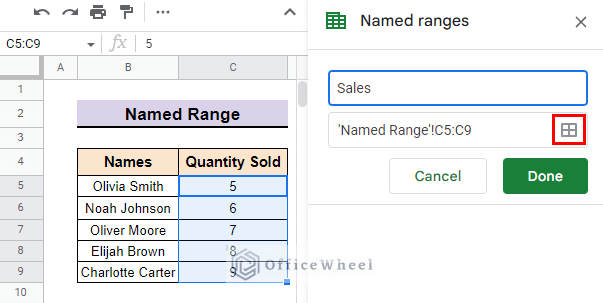
- Finally, press Done and the selected range is named according to your choice.

3 Simple Approaches to Use VLOOKUP with Named Range in Google Sheets
The VLOOKUP function lets you look for a particular value down the first column in a range of cells. VLOOKUP can be used with Named Range to have a cleaner feel about the formula and it can help you by saving lots of precious time.
1. From Same Worksheet
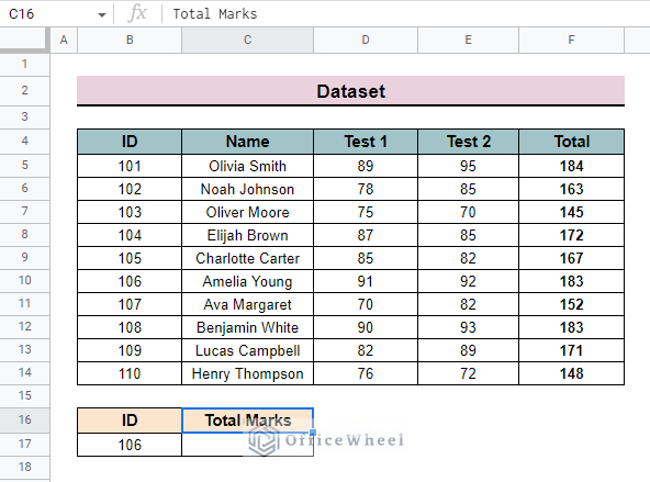
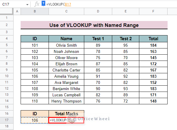
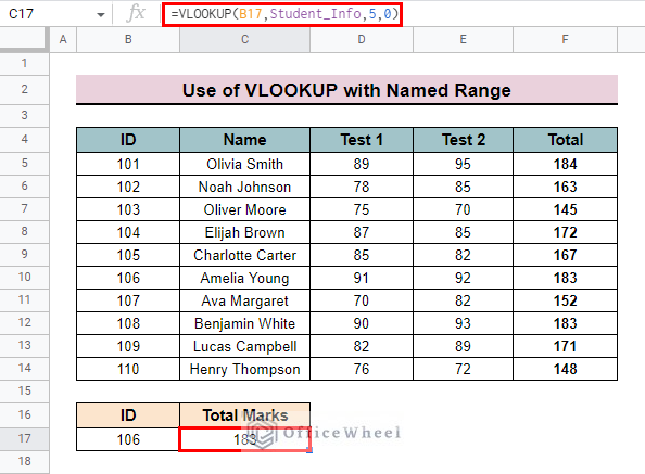
We use the following dataset with Student ID, their Name, marks obtained by the students in Test 1 and Test 2, and the Total Marks obtained by each of the students. We will use this table to show the Total Marks obtained by each student in a separate cell.
Steps:
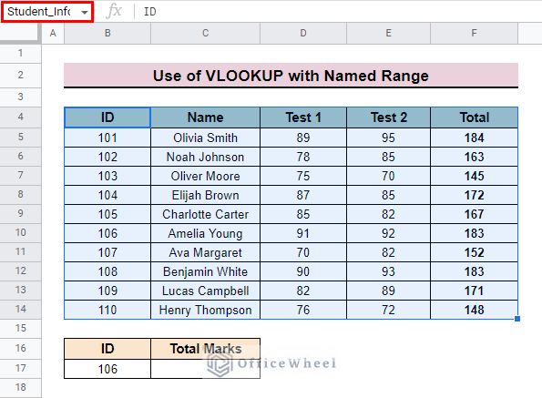
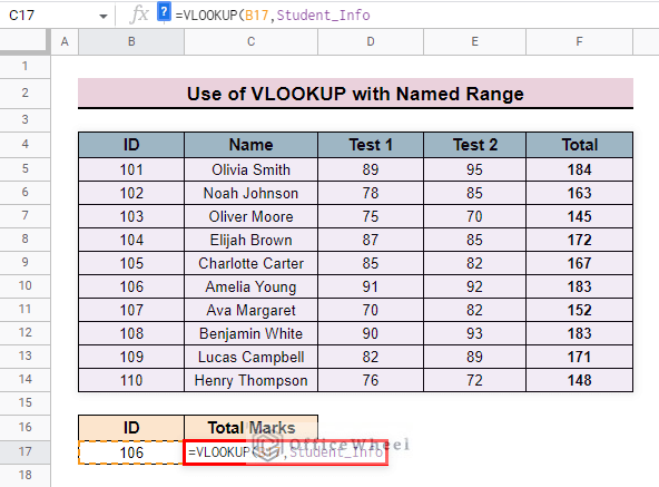
- First, name the entire table by following the steps shown above. We name the table Student_Info.
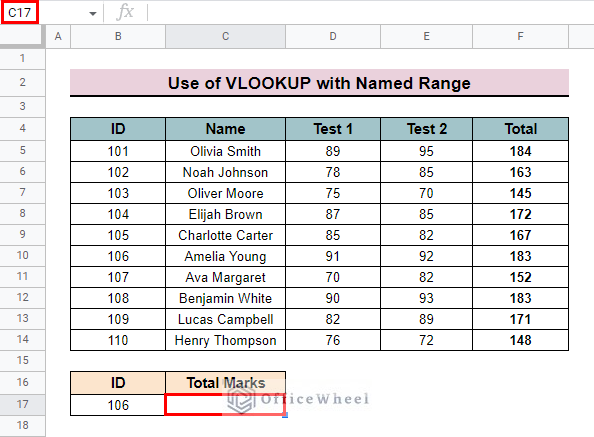
- Then, go to the cell where you want to show the lookup value. We go to cell C17 in our example.
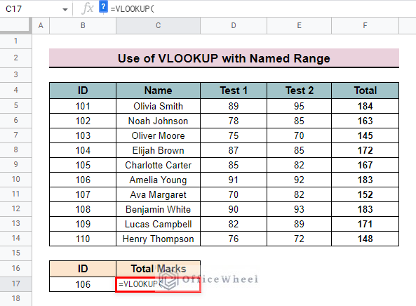
- After that, insert the VLOOKUP function.
- Then, type the value you want the formula to look for. We kept the ID we want to look for in a different cell and so we type that cell reference which is B17.
- Now, type the name that you assigned as the name for the range in place of the range parameter of the VLOOKUP We type Student_Info (the named range) in our example.
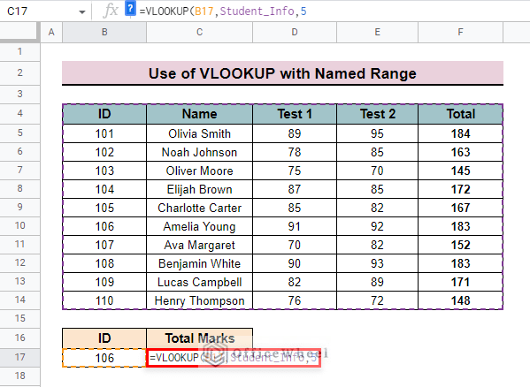
- After that, type the column number whose data you want the formula to return if the VLOOKUP finds a match. We type 5 as we want the formula to return the Total Mark obtained by the students which are in the 5th column of our data table.
- Type 0 or FALSE as you want an exact match for the value.

- Finally, close the parenthesis for the VLOOKUP function and press ENTER to close up the formula and show the result. This is what the final formula looks like:
=VLOOKUP(B17,Student_Info,5,0)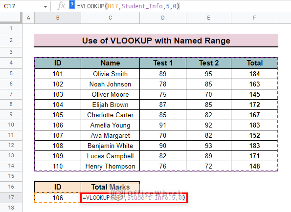
- We press ENTER to show the mark obtained by ID 106.
Read More: How to Check If Value Exists in Range in Google Sheets (4 Ways)
Similar Readings
- Google Sheets Vlookup Dynamic Range
- [Fixed!] Google Sheets If VLOOKUP Not Found (3 Suitable Solutions)
- How to Use VLOOKUP Function for Exact Match in Google Sheets
- Alternative to Use VLOOKUP Function in Google Sheets
- How to Use VLOOKUP with Drop Down List in Google Sheets
2. From Another Sheet
Named Range can be a useful tool to use when using VLOOKUP to import and show data from another sheet from the same workbook.
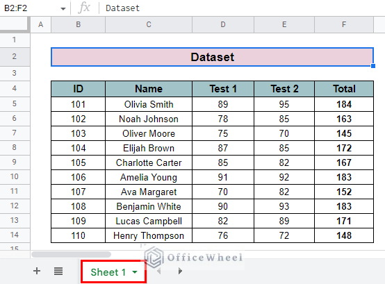
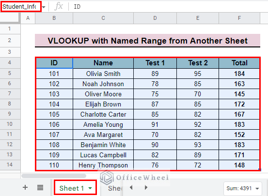
Suppose we have the data table used in the previous method in Sheet 1. We will show the Total Marks obtained by each student in Sheet 2 of the same workbook.
Steps:
- First, name the entire table of Sheet 1 by following the steps shown above. We name the table Student_Info.
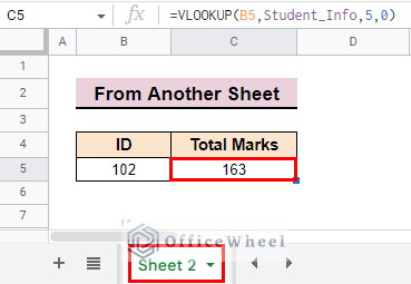
- Then, go to the cell of the new sheet where you want the Total Mark to appear. We go to cell C5 of Sheet 2.
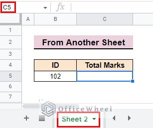
- Type the following Formula:
=VLOOKUP(B5,Student_Info,5,0)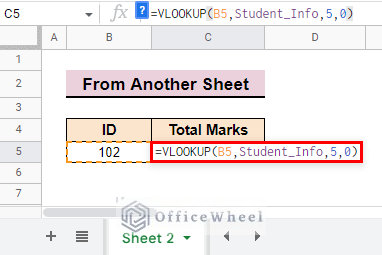
The above VLOOKUP formula will look like this without using the named range:
=VLOOKUP(B5,'Sheet 1'!B4:F14,5,0)This is the main benefit of using named ranges.
Formula Explanation:
- B5 is the value that we want to look for.
- Student_Info is the name of the range from where we want to look for the data.
- 5 is the column number of the table whose data we want the formula to return.
- 0 or FALSE is used because we want an exact match for our data.
- Finally, press ENTER to show the result in cell C5 of Sheet 2.
Read More: How to VLOOKUP from Another Sheet in Google Sheets (2 Ways)
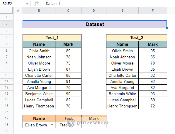
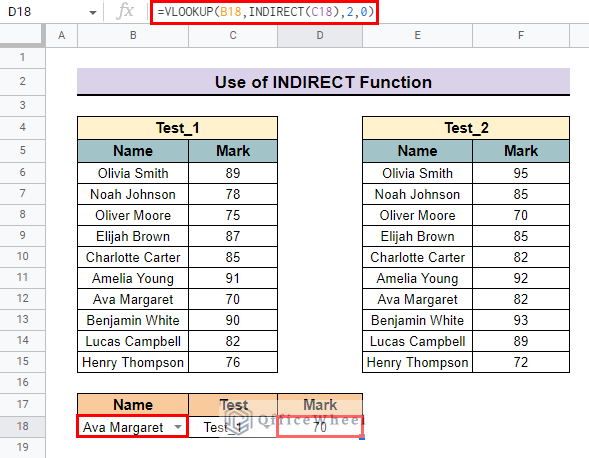
3. Use of INDIRECT Function
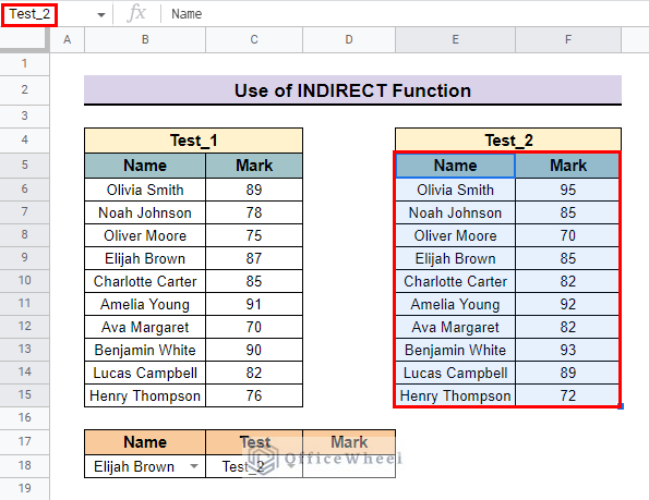
We use the Named range in place of the range in the VLOOKUP function. The INDIRECT function can be used to indicate the Named range in place of the range in the VLOOKUP function. We have a dataset with two different tables. Table Test_1 contains the marks obtained by the students in Test 1 and table Test_2 contains the marks obtained by the Students in Test 2. We kept the names of students in cell B18 by using a data validation drop-down list. We kept the different test types in cell C18.
Steps:
- First, name the tables by following the steps shown above. We named the first range Test_1.
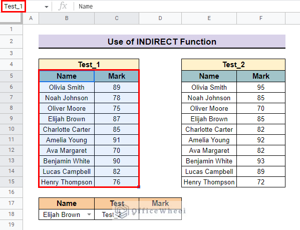
- And named the second range Test_2.
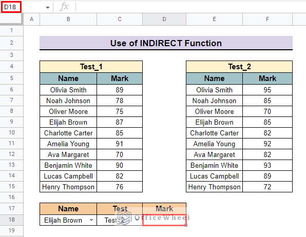
- Then, go to the cell where you want the Mark of the tests to appear. We go to cell D18 in our example.
- Then, type the following formula:
=VLOOKUP(B18,INDIRECT(C18),2,0)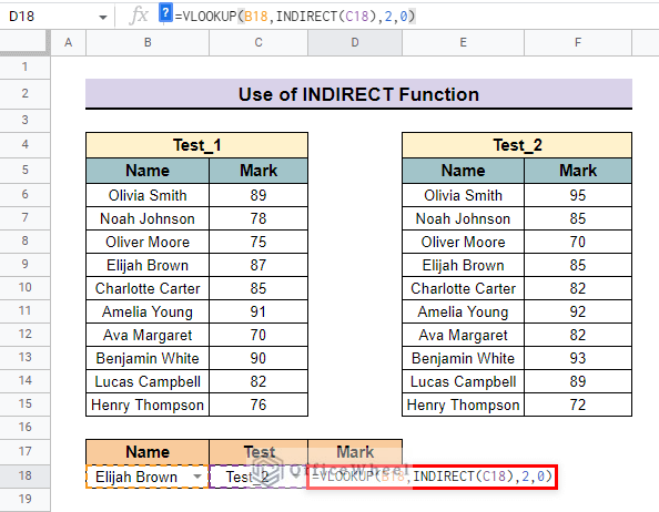
Formula Explanation:
- B18 is the value that we want to look for.
- INDIRECT(C18) is the range of the two tables from where we want to look for the data.
- 2 is the column number of the table whose data we want the formula to return.
- 0 or FALSE is used because we want an exact match for our data.
- Finally, press ENTER to show the result.
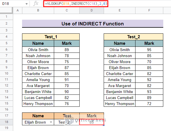
- We can select different students’ names from the drop-down list in cell C18 and select between two different test types from cell B18. The result will be changed accordingly.
Read More: Highlight Cell If Value Exists in Another Column in Google Sheets
Things to Remember About Named Ranges
- You cannot use space between words or letters while naming a range.
- You cannot use duplicate names for Named Range in a workbook.
- The name for Named ranges cannot contain anything other than numbers, letters, and underscores.
- You cannot use the reference of a cell or a range to name a range. For example, A5, D6:D11, cannot be used as a Named range.
Conclusion
In this article, we showed you what Named range is and how you can use VLOOKUP with named ranges in Google Sheets. Keep practicing the methods that we have shown here for a better understanding of the concept. We hope this article was useful to you to help you.
Also, check out other articles on OfficeWheel to keep on improving your Google Sheets work knowledge.
Related Articles
- How to Use Wildcard in Google Sheets (3 Practical Examples)
- How to Use Nested VLOOKUP in Google Sheets
- How to VLOOKUP for Partial Match in Google Sheets
- VLOOKUP Error in Google Sheets (with Quick Solutions)
- Combine VLOOKUP and HLOOKUP Functions in Google Sheets
- Create Hyperlink to VLOOKUP Cell in Multiple Rows in Google Sheets
- VLOOKUP with IMPORTRANGE Function in Google Sheets
- How to Use VLOOKUP for Conditional Formatting in Google Sheets