Google Sheets Conditional Formatting with INDEX-MATCH

Conditional formatting is an excellent tool in Google Sheets to highlight specific data. In Google Sheets, the INDEX and MATCH functions allow you to use effective and tricky conditional formatting. It helps to visualize relevant data in a large datasheet easily. This article will demonstrate how to apply conditional formatting with the INDEX-MATCH functions in Google Sheets.

A Sample of Practice Spreadsheet

You can download the practice spreadsheet from the download button below.

2 Ideal Examples of Conditional Formatting with INDEX-MATCH in Google Sheets

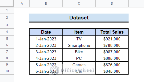
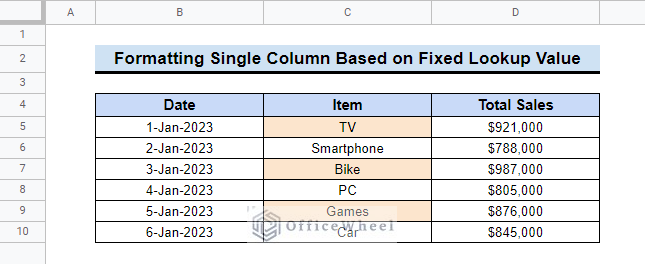
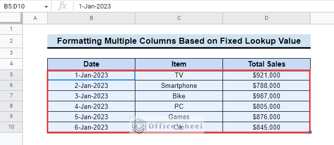
Let’s assume, we have a dataset that contains the total sales of some products on some particular days.

We will apply conditional formatting on this dataset using the INDEX-MATCH functions in Google Sheets. There are multiple criteria to do that. Follow the article to learn them.

1. Formatting Based on Fixed Lookup Value

First, you can apply conditional formatting with INDEX-MATCH based on a fixed lookup value. You can do this to a single column or multiple columns. Read along to learn the methods.

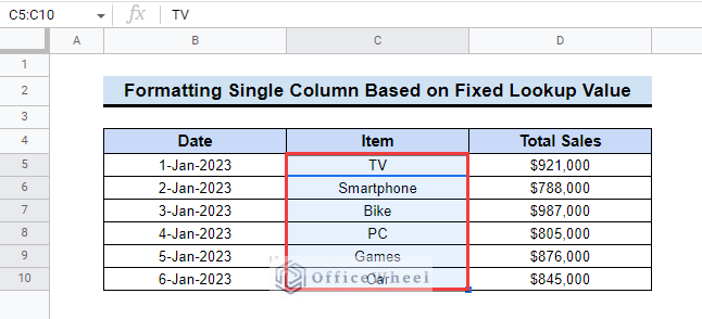
1.1 Formatting Single Column

You can easily format a single column based on a fixed lookup value. Follow the steps below to do that by yourself.

📌 Steps:

• At the very beginning, select the cell range C5:C10 in the dataset.

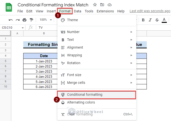
• Next, click on the Format option from the top menu bar.
• Then, select the Conditional formatting option from the dropdown list.

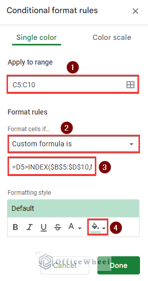
• After that, a pane named Conditional format rules will appear on the right side of the Google Sheets.
• Then, you will see the selected range under the Apply to range. Or, you can set a new range.
• Following, choose the “Custom formula is” from the “Format cells if…” option.
• Next, insert the following formula in the box.

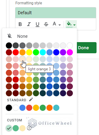
• Later, click on the fill color icon from the Formatting style.

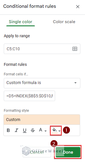
• Next, choose any color from the list of colors to highlight the formatted cells.

• Now, select the Done button.

• Finally, you will see a highlighted datasheet like the following image.

Read More: Use of Google Sheets INDEX MATCH in Multiple Columns

1.2 Formatting Multiple Columns

You can also apply conditional formatting to multiple columns based on a fixed lookup value. The steps to do that are mentioned below.

📌 Steps:

• First, select the cell range B5:D10 to apply conditional formatting.

• Now, just like before, follow the steps in the following image and insert the below-mentioned formula in the formula box.

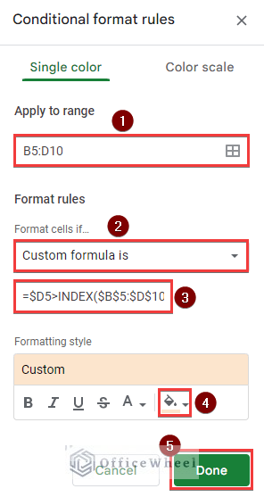
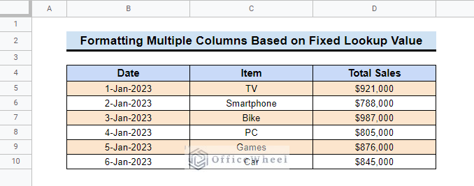
• Finally, you will get the following result.

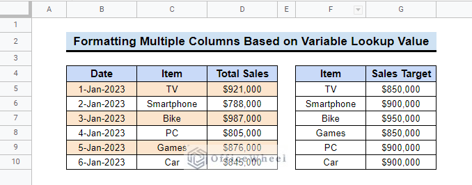
2. Formatting Based on Variable Lookup Value

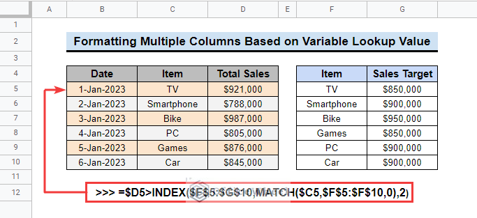
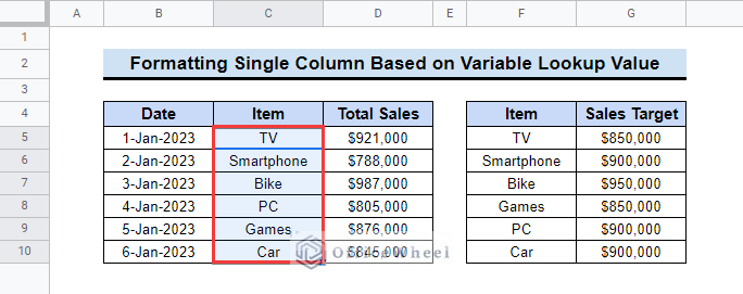
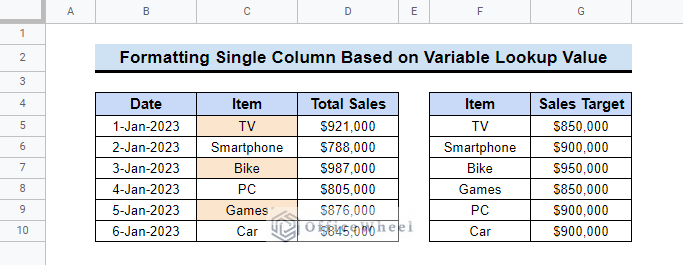
If you want to apply conditional formatting based on variable lookup value, you can do that too. Here are the methods to do that. Here, another data table is given. This table has the same products, and the Sales Target is mentioned in the next column. You can compare the data and apply formatting to highlight them.

2.1 Formatting Single Column

You can format a single column based on a variable lookup value. The easy steps to do that are mentioned below.

📌 Steps:

• First, select the cell range C5:C10 in the dataset.

• Then, like the above methods, go to Format >> Conditional formatting.
• After that, you will see the range you already selected in the Apply to range.
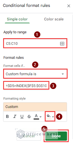
• Next, in the Format rules option, enter the following formula in the Custom formula is box.

• Subsequently, follow the next number of steps.

• Eventually, it will return the dataset like the below image.

Similar Readings 

• Combine VLOOKUP and HLOOKUP Functions in Google Sheets
• How to Create Conditional Drop Down List in Google Sheets
• Match Multiple Values in Google Sheets (An Easy Guide)

2.2 Formatting Multiple Columns

It is easy to format multiple columns based on a variable lookup value. Follow the steps then you can also do that.

📌 Steps:

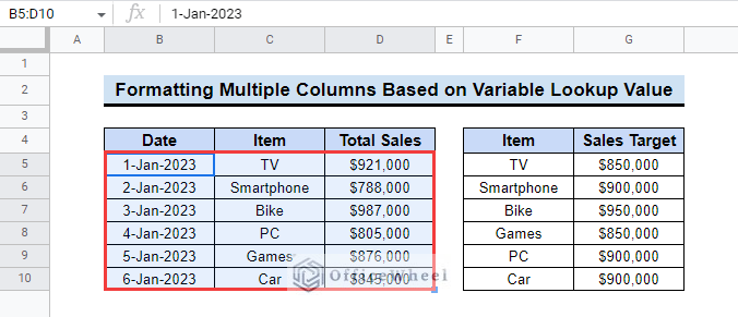
• Initially, select the B5:D10 cell range.

• Then, like before, go to Format >> Conditional formatting to apply conditional formatting.
• Next, enter the following formula in the Format rules option of the Conditional format rules window. Follow step number 2 in the next image.
• Subsequently, insert the formula in the Custom formula is box.

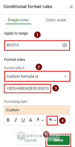
• Finally, the selected range will be highlighted according to applied conditional formatting.

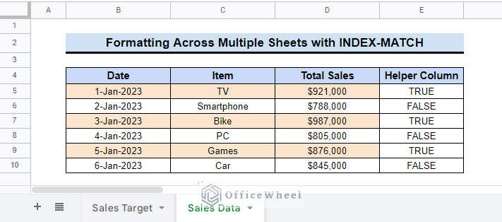
How to Apply Conditional Formatting with INDEX-MATCH from Another Sheet in Google Sheets

You can also use the INDEX-MATCH combination for another sheet and apply conditional formatting. Suppose the sales target is mentioned in another sheet named Sales Target.

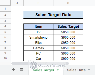
You will use this data to index match and then apply conditional formatting.  Follow the steps below to be able to do that.

📌 Steps:

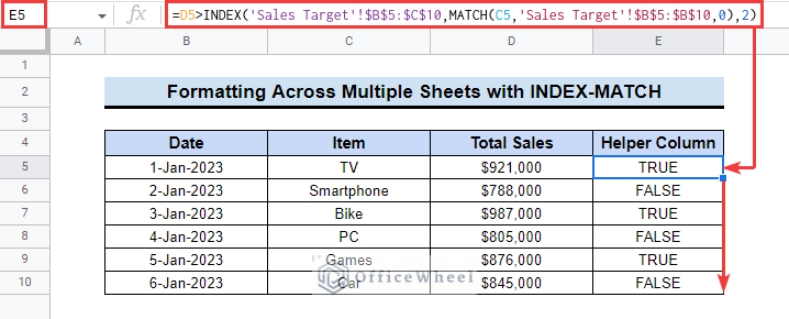
• First, select cell E5 and apply the following formula.

• Then drag the fill handle down to cell E10.

• Select cell range B5:D10 and apply conditional formatting following any of the above methods with the above formula in the formula box.

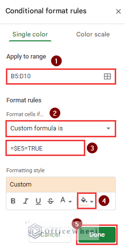
• Finally, the dataset will look like this.

Read More: [Fixed!] INDEX MATCH Is Not Working in Google Sheets (5 Fixes)

Things to Remember

When you apply conditional formatting to multiple columns, be careful to use the mixed cell reference. Otherwise, the formatting won’t work.

Conclusion

We have tried to show you the uses of Conditional Formatting with Index Match in Google Sheets. Hopefully, the examples above will be enough for you to understand the applications of the function. Please use the comment section below for further queries or suggestions. You may also visit our OfficeWheel blog to explore more about Google Sheets.

Related Articles

• Google Sheets HLOOKUP to Return Column (3 Simple Ways)
• How to VLOOKUP Left in Google Sheets (4 Simple Ways)
• Alternative to Use VLOOKUP Function in Google Sheets
• How to Create Dependent Drop Down List in Google Sheets
• Find All Cells With Value in Google Sheets (An Easy Guide)