We often need to find specific information from a dataset in Google Sheets. We use the VLOOKUP function for vertical search and HLOOKUP to search any data placed horizontally. However, there are times when we need to search for specific information using both vertical and horizontal data. In these instances, we need to combine the VLOOKUP and HLOOKUP functions in Google Sheets. In this article, we will show some methods and alternatives to do this task in Google Sheets.
A Sample of Practice Spreadsheet
You can download the practice spreadsheet from the download button below.
2 Easy Ways to Combine VLOOKUP and HLOOKUP Functions in Google Sheets
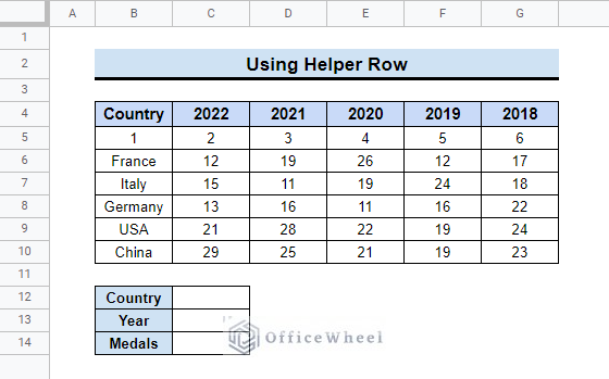
Let’s assume we have a dataset that contains the number of medals some countries achieved in a tournament in some particular years.
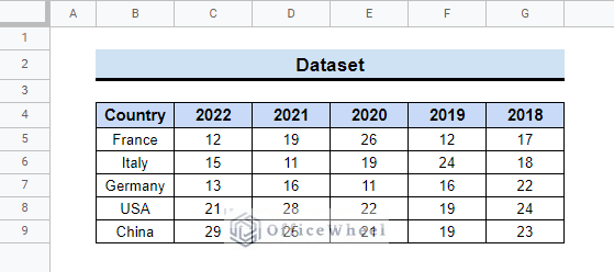
Now from this dataset, if you want to look for the data that a particular team achieved how many medals in a particular year then you will need to search for data from both the rows and columns. This is when you will need to combine the VLOOKUP and HLOOKUP functions in Google Sheets. Follow this article to learn how to do that.
1. Using Helper Row
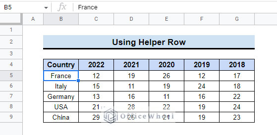
The first method you can use is to add a helper row to the dataset. You can add a new row and use HLOOKUP to search for data from the rows. Follow the steps below to do it by yourself.
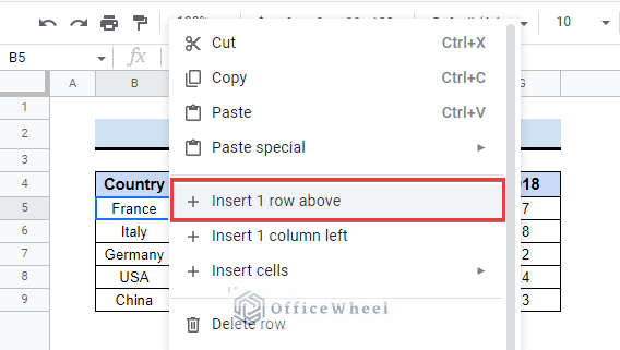
- First, select cell B5 in the dataset. You need to insert a row above this row.
- Then, right-click on the mouse to see the context menu. And, choose Insert 1 row above from there.
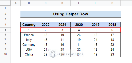
- After that, you will see a new row added to the dataset. Now, number the cells in that row starting from 1.
- Next, make a small data table for the Country, Year, and Medals like the following image.
- Now, insert the below-mentioned formula in cell C14. And give a Country name and Year input in the blank cells. You will get the medal number in C14.
=VLOOKUP(C12,B4:G10,(HLOOKUP(C13,C4:G5,2,FALSE)),FALSE)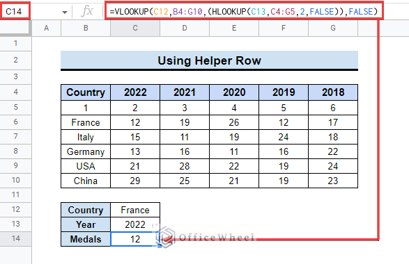
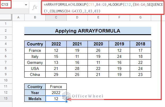
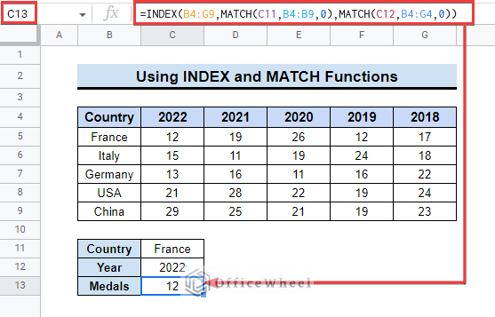
Formula Breakdown: Read More: Alternative to Use VLOOKUP Function in Google Sheets Another way to combine VLOOKUP and HLOOKUP in Google Sheets is to use the ARRAYFORMULA function with these functions. The ARRAYFORMULA function can return multiple results from an array or multiple rows and columns. This will eliminate the need to add a helper row in the first place. Follow the steps below to learn how to use these functions together with the ARRAYFORMULA function to look for data using both row and column information. Read More: Match from Multiple Columns in Google Sheets (2 Ways) There is an alternative to combining the VLOOKUP and HLOOKUP Functions in Google Sheets. You can use the INDEX and the MATCH functions to do the same thing. The INDEX function returns data from particular cells or a range of cells input. Additionally, the MATCH function returns the location of an item within a range that corresponds to a given value. Follow the steps to use the INDEX-MATCH functions to search data using rows and columns. Formula Breakdown:
Read More: Find All Cells With Value in Google Sheets (An Easy Guide) We have tried to show you the method to combine VLOOKUP and HLOOKUP functions in Google Sheets. Hopefully, the examples above will be enough for you to understand the applications of the function. Please use the comment section below for further queries or suggestions. You may also visit our OfficeWheel blog to explore more about Google Sheets.
2. Applying ArrayFormula
=ARRAYFORMULA(VLOOKUP(C11,B4:G9,HLOOKUP(C12,{B4:G4;SEQUENCE(1,COLUMNS(B4:G4))},2,0),0))
Alternative to Combining VLOOKUP and HLOOKUP Functions in Google Sheets
=INDEX(B4:G9,MATCH(C11,B4:B9,0),MATCH(C12,B4:G4,0))
Things to Remember
Conclusion
Related Articles