Using INDEX MATCH in Google Sheets – A Deep Dive

Today, we will look at the use of INDEX MATCH in Google Sheets. This amazing combination of functions is available in both Excel and Google Sheets. So, if you have been using Excel or have the fundamental expertise of using spreadsheets, you should feel right at home.

This article should provide you with an in-depth guide on how to use INDEX MATCH.

Let’s get started.

INDEX and MATCH Basics

MATCH

We start off with the more commonly used of the two, the MATCH function. The MATCH function returns the position of the cell that matched the given “key” or value in a range.

The syntax:

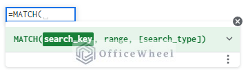
Breakdown:

• search_key: It is the value we search for in the given range.
• range: The range of cells on which the search and match are performed.
• [search_type]: Optional. It is 1 by default.
  • 1: Assumes that the search range is sorted in ascending order.
  • 0: Makes the function go for an exact match assuming that the range is not sorted.
  • -1: Assumes that the range is sorted in descending order.

Example:

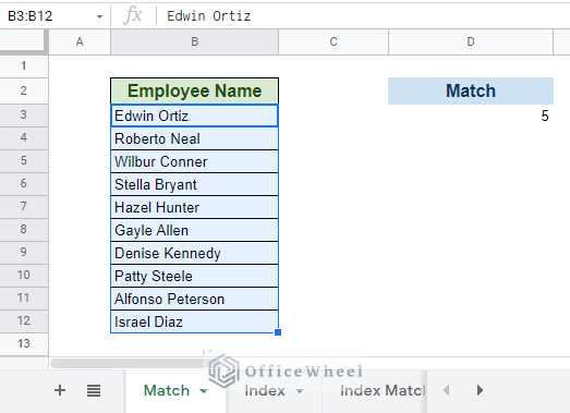
In the following list of Employee Names, we will perform a MATCH to find Hazel Hunter.

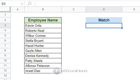
Our formula at D3 will be:

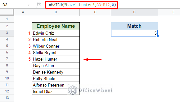
Our MATCH function recognizes that the name Hazel Hunter was at the 5^th position (or index) in our range.

We put 0 as the search_type as we wanted an exact match position in our range. Without the 0, our function would have returned just the row number of the match, which is 7.

INDEX

Next up, we have the INDEX function. This function returns the content of the cell (or cells around it)

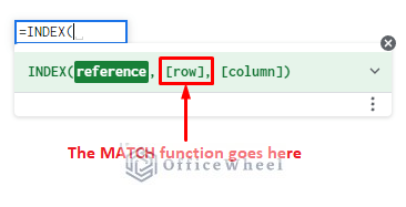
The syntax:

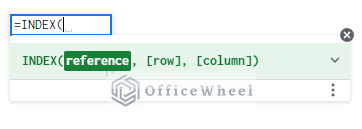
Breakdown:

• reference: The range of cells to be checked
• [row]: Optional. 0 by default. Returns the index of the row within the range reference.
• [column]: Optional. 0 by default. Returns the index of the column within the range reference.

Example:

We will be returning the 5^th row index from the range of values from the following table.

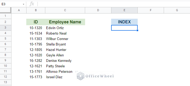
Since row and column references are optional, we will try with just the row reference first. Our formula:

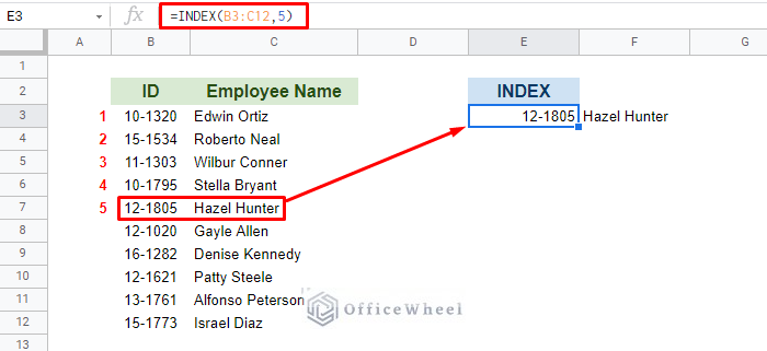
As you can see, the entire row within the reference range was returned.

Now, if we specify the column index:

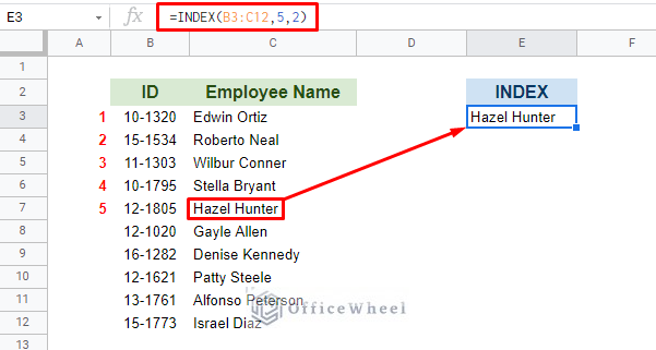
Only one pin-pointed value was returned.

The opposite can happen if we leave the row index blank. In the case of this table, we would have just gotten the list of names.

You may have noticed that the INDEX function is much like finding coordinates, making it very easy to use.

Combining INDEX and MATCH Functions

Since the MATCH function returns the relative position (index) of the given value, it can be substituted for the row index in the INDEX function.

So, our INDEX MATCH formula becomes:

In the following section, we will look at two fundamental ways in which we can use this amazing formula and later, how it is better than its old counterpart, the VLOOKUP function.

Read More: Combine VLOOKUP and HLOOKUP Functions in Google Sheets

2 Fundamental Ways to Use INDEX MATCH in Google Sheets

1. INDEX MATCH Single Criteria (Single Column Reference)

For our first example, we will be working with a single criterion (single column match) for our INDEX MATCH.

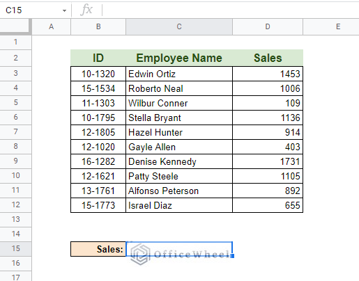
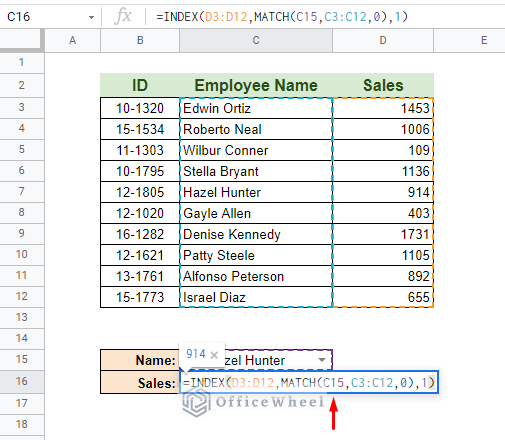
In the following worksheet, we will extract the number of Sales done by Hazel Hunter.

Step 1: We open the INDEX function and input the range for the Sales column data.

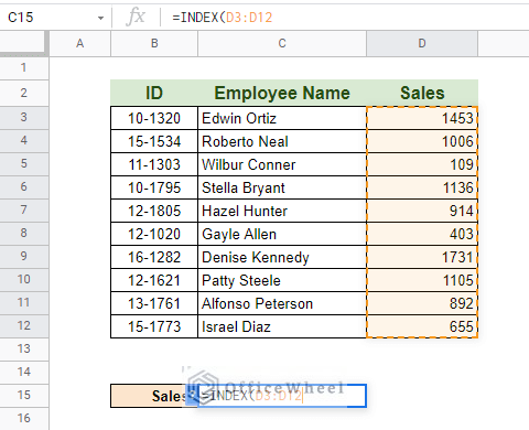
Step 2: We input the MATCH function to find the row index for Hazel Hunter.

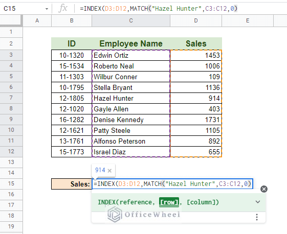
Step 3: Close off the formula with a 1 for the column index. Our formula:

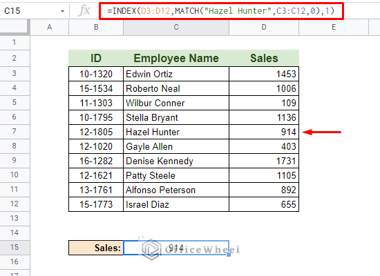
It’s as simple as that!

You can also use a cell reference to get what you need.

To create an in-cell drop-down menu follow this link.

Similar Readings  

• [Fixed!] INDEX MATCH Is Not Working in Google Sheets (5 Fixes)
• How to Create Conditional Drop Down List in Google Sheets

Case-Sensitive Lookup (ArrayFormula, FIND)

Now let’s have a look at this table.

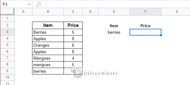
We have two different inputs of “Berries”, one starting with a capital and the other not.

In this case, we have to modify our formula to select the correct case item from our list and display its price.

Step 1:

We will apply the FIND function on the Item column to return the correct price. It is a case-sensitive formula.

Any matches found using this function will return 1.

Step 2:

The MATCH function will search for this “1” in the Item column.

Step 3:

We incorporate this in the INDEX function with our return value coming from the Price column.

Step 4:

Press CTRL+SHIFT+ENTER or enclose the INDEX MATCH formula within ARRAYFORMULA. This will allow the FIND function to search in more than one cell (array).

Our final formula:

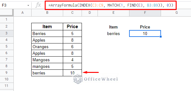
Alternative:

You can replace the FIND function with EXACT and replace the 1 with TRUE in the MATCH function.

INDEX MATCH From a Different Worksheet

The INDEX MATCH formula has the advantage of not having to add any complicated modifications when we look to import values or criteria from another worksheet.

We can simply add the reference to a separate worksheet, and we are good to go!

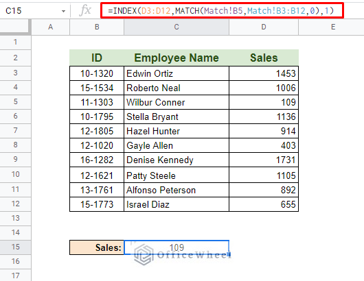
Our MATCH criteria come from the worksheet called Match.

2. INDEX MATCH Multiple Criteria (Multiple Column Reference)

So far, we have worked with only a single column for our INDEX range. Not only that but there was also a single MATCH criterion.

The INDEX MATCH formula allows us to do much more than that, a two-dimensional lookup with multiple criteria.

To show this, we will be extracting the ID number of the given employee mentioned in cell C15.

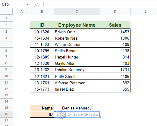
So, we have two MATCH criteria:

1. The Name: MATCH(C15,C3:C12,0)
2. The Column Criteria: MATCH(B16,B2:D2,0)

Note: The Column Criteria is basically searching the table headers.

Thus, our INDEX MATCH formula will be:

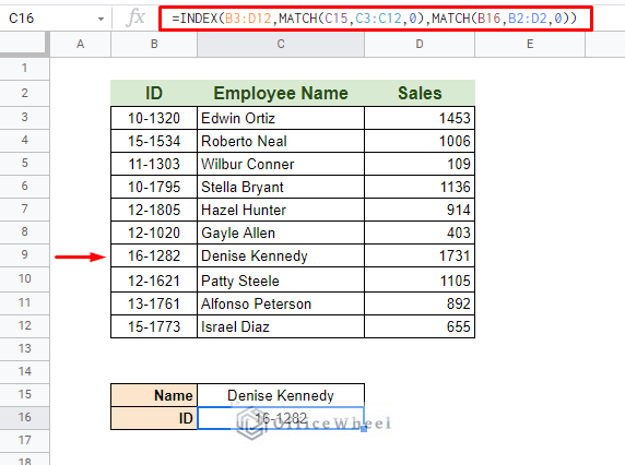
Formula Breakdown:

• range: B3:D12
• row index: MATCH(C15,C3:C12,0)
• column index: MATCH(B16,B2:D2,0)

Now, even if we change the name in cell C15, we will still get the correct ID:

Read More: Match Multiple Values in Google Sheets (An Easy Guide)

Why is INDEX MATCH A Better Alternative to VLOOKUP?

Reading this article so far, you might be thinking that these objectives we have accomplished can also be done with the VLOOKUP function, right?

Yes and No.

There are a few advantages that the INDEX MATCH combination has over the VLOOKUP function:

• Looking both ways: With the INDEX MATCH formula, we can lookup values on both left and right sides of the search column. Whereas VLOOKUP only looks toward the left of the column.
• Allows changes: Since INDEX MATCH accesses only the cell references, adding or moving columns will not affect our searches.
• Takes text cases into account: A slight modification can allow the INDEX MATCH function to search for case-sensitive searches. See method 1.
• Can take multiple criteria: INDEX MATCH can work with multiple conditions from tables of the same or different worksheets with ease. See method 2.

Final Words

INDEX Match is a wonderful combination of functions for both Excel and Google Sheets. Its depth of use is extraordinary all the while keeping things simple and easy to understand. This makes this function a great choice for beginners and professionals alike.

We hope that with the help of our article, you will now be able to implement INDEX MATCH into your daily work.

Feel free to leave any queries or advice you might have in the comments below.

Related Articles

• Google Sheets Conditional Formatting with INDEX-MATCH
• Google Sheets HLOOKUP to Return Column (3 Simple Ways)
• Find All Cells With Value in Google Sheets (An Easy Guide)
• How to Create Dependent Drop Down List in Google Sheets
• Find Cell Reference in Google Sheets (2 Ways)
• INDEX-MATCH with Multiple Criteria in Google Sheets (Easy Guide)
• Match from Multiple Columns in Google Sheets (2 Ways)