The VLOOKUP is one of the most useful options in Google Sheets and Excel. This option is useful for searching and extracting information from a large dataset. Several functions like the VLOOKUP, XLOOKUP, or a combination of INDEX and MATCH functions, etc. can perform the VLOOKUP operation. While making datasheets in Google Sheets or Excel, we often use date values. So, a ques arrives, “Can we apply VLOOKUP by Date?”. The answer is “Yes”. Here, in this article, I’ll demonstrate 2 examples to apply VLOOKUP by date in Google Sheets.
A Sample of Practice Spreadsheet
You can copy our practice spreadsheets by clicking on the following link. The spreadsheets contain an overview of the datasheet and an outline of the described examples to apply VLOOKUP by date.
2 Helpful Examples to Apply VLOOKUP by Date in Google Sheets
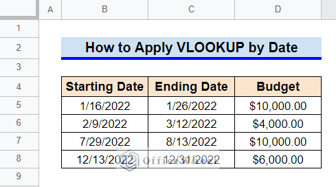
First, let’s get familiar with our dataset. The dataset contains starting and ending dates of several projects and the estimated budget for these projects. We’ll extract the estimated budget data from the dataset based on date values. Note that the dataset here is sorted.
Example 1: Using VLOOKUP by Date
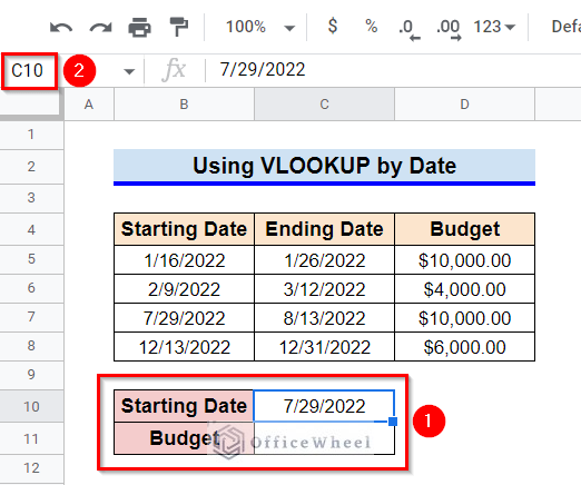
Here, we’ll do a simple VLOOKUP based on a date value. We have to modify our datasheet like the following and enter any starting date from Column B in Cell C10.
Steps:
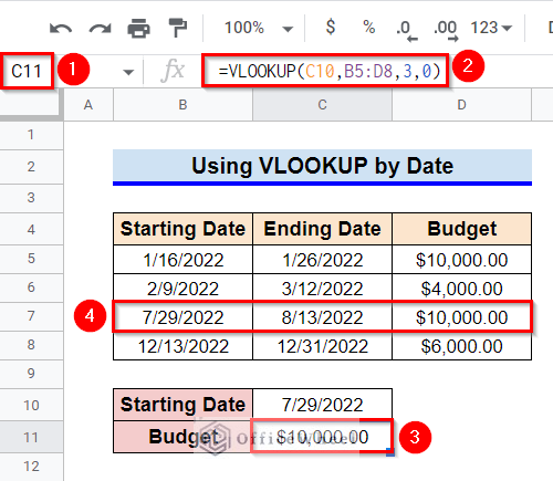
- First, select Cell C11.
- Then, type in the following formula:
=VLOOKUP(C10,B5:D8,3,0)- Finally, press Enter key to get the required result.
Read More: Group Dates in a Google Sheets Pivot Table (An Easy Guide)
Example 2: Applying VLOOKUP Between Two Dates
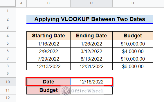
In the previous example, we used the exact date for looking up. But can we use any random date between two specific values? Yes, we can. Go through the following three examples to know how.
Also, instead of a starting date, we require a random date now. Therefore, modify the datasheet as follows:
Example 2.1: Implementing for Sorted Date Range
The VLOOKUP function will select the nearest match when it can’t find an exact match for the search key in a sorted data range.
Steps:
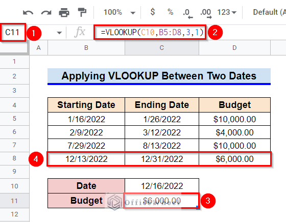
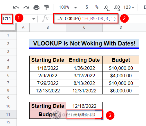
- First, select Cell C11.
- Afterward, type in the following formula:
=VLOOKUP(C10,B5:D8,3,1)- Finally, press Enter key to get the required result. As you can see, the Date 12/16/2022 doesn’t exactly match with any of the values in range B5:C8. But it falls between the dates 12/13/2022 and 12/31/2022. Hence, the VLOOKUP function has extracted data from Row 8.
Read More: Google Sheets Vlookup Dynamic Range
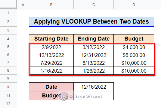
Example 2.2: Employing for Unsorted Date Range
The date range was sorted in the previous example. But what happens when the dataset is not sorted? Will the previous method work if the data range is not sorted? The answer is No, it won’t. For example, consider the following modification in the dataset. The date range is now unsorted.
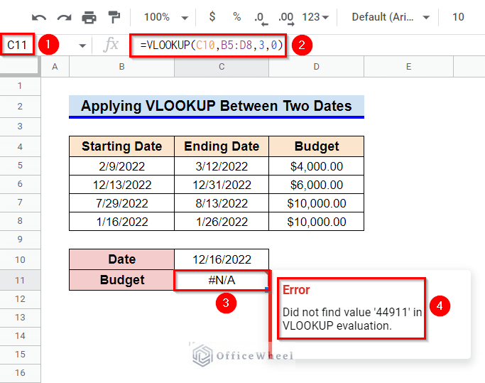
Now, if we apply a formula like the previous method, we see an #N/A error. However, you can still perform a VLOOKUP using a combination of the ARRAYFORMULA and LOOKUP functions.
Steps:
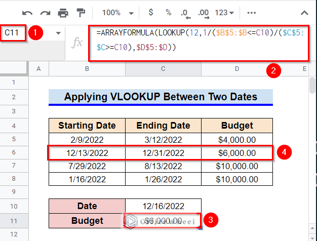
- First, select Cell C11.
- After that, type in the following formula:
=ARRAYFORMULA(LOOKUP(12,1/($B$5:$B<=C10)/($C$5:$C>=C10),$D$5:$D))- Finally, press Enter key to get the required value.
Formula Breakdown
- LOOKUP(12,1/($B$5:$B<=C10)/($C$5:$C>=C10),$D$5:$D)
First, the LOOKUP function searches for a random value of 12 provided as the search key in the search range. The search range here will be 1 or #DIV/0! error. The LOOKUP function will select the value for which it will find the last match. Finally, it returns the value from the second row of the result range D5:D.
- ARRAYFORMULA(LOOKUP(12,1/($B$5:$B<=C10)/($C$5:$C>=C10),$D$5:$D))
The ARRAYFORMULA function helps to deal with the arrays in LOOKUP function arguments.
Read More: How to Use ARRAYFORMULA with VLOOKUP in Google Sheets
Example 2.3: Combining VLOOKUP and SORT Functions
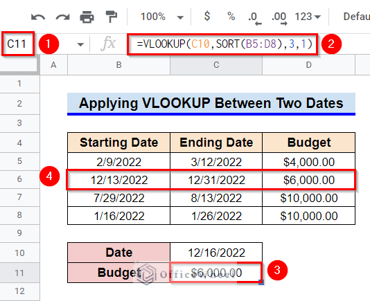
If you find the previous method a little complex, you can simply combine the SORT function with the VLOOKUP function to virtually sort the date range.
Steps:
- First, select Cell C11.
- Afterward, type in the following formula:
=VLOOKUP(C10,SORT(B5:D8),3,1)- Finally, press Enter key to get the required result.
Formula Breakdown
- SORT(B5:D8)
First, the SORT function sorts the rows of the range B5:D8.
- VLOOKUP(C10,SORT(B5:D8),3,1)
Afterward, the VLOOKUP function will return the content of the third column in the sorted range where the closest match is found for the search key in Cell C10.
Read More: Combine VLOOKUP and HLOOKUP Functions in Google Sheets
Similar Readings
- How to Use VLOOKUP with IF Statement in Google Sheets
- VLOOKUP Multiple Columns in Google Sheets (3 Ways)
- How to Use ARRAYFORMULA with IF Function in Google Sheets
- Highlight Cell If Value Exists in Another Column in Google Sheets
- How to Use Formula to Highlight Duplicates in Google Sheets
What to Do When VLOOKUP Is Not Working with Dates in Google Sheets
There can be various reasons behind the VLOOKUP function not working with date ranges. We have already acknowledged one of the reasons in Example 2.2 where the dataset was not sorted. Example 2.2 and Example 2.3 provided solutions for that problem. Here, we will discuss a different problem.
As we have seen in Example 2.1, the VLOOKUP function selects the nearest value if an exact match is not found in a sorted dataset. But in the following dataset, an #N/A error is returned for that similar formula.
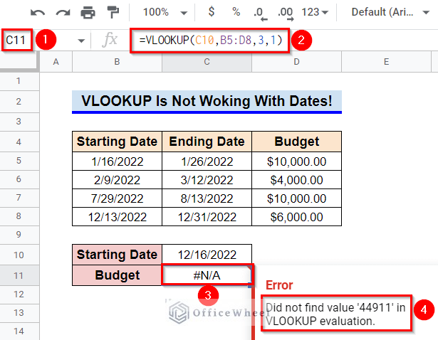
The reason for the error is that the date range is formatted as “Plain Text” instead of “Date”. There can be reasons behind formatting the dates as plain text values. So, can we do VLOOKUP without changing the format? The answer is a resounding Yes! We can join the INDEX, MATCH, and DATEVALUE functions to get the required result. However, if the plain text format isn’t important, then simply changing the data format will work for applying the VLOOKUP function. We will discuss both of these solutions below.

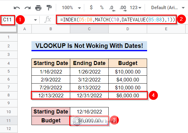
Solution 1: Using DATEVALUE Function
- First, select Cell C11.
- Then, type in the following formula-
=INDEX(D5:D8,MATCH(C10,DATEVALUE(B5:B8),1))- Finally, press Enter key to get the required result.
Formula Breakdown
- DATEVALUE(B5:B8)
First, the DATEVALUE function converts the date strings in the range B5:B8 into date values.
- MATCH(C10,DATEVALUE(B5:B8),1)
Afterward, the MATCH function returns the relative position of the cell in range B5:B8 where a match is found for the search key provided in Cell C10.
- INDEX(D5:D8,MATCH(C10,DATEVALUE(B5:B8),1))
Finally, the INDEX function returns the content of the subsequent cell in range D5:D8, where it finds a match for range B5:B8.
Read More: How to Use the DATEVALUE Function in Google Sheets (An Easy Guide)
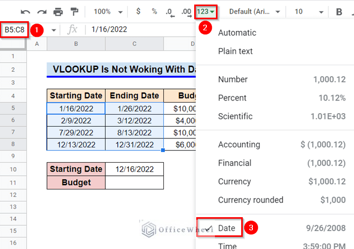
Solution 2: Applying Date Format
- First, select the range B5:C8 and change the data format to “Date”.
- Afterward, type in the following formula in Cell C11:
=VLOOKUP(C10,B5:D8,3,1)- Finally, press Enter key to get the required result.
Read More: How to Format Date with Formula in Google Sheets (3 Easy Ways)
Things to Be Considered
- The VLOOKUP function will select the nearest match when it can’t find an exact match for the search key in a sorted data range.
- The combination of INDEX and MATCH functions will work only if we provide a sorted date range.
- The LOOKUP function will select the value for which it will find the last match.
- The VLOOKUP function can’t execute properly when it can’t find an exact match in an unsorted dataset.
- Remember to format both the lookup value and range as a date.
Conclusion
This concludes our article to learn how to apply VLOOKUP by date in Google Sheets. I hope the described examples were sufficient for your requirement. Feel free to leave your thought on the article in the comment box. Visit our website OfficeWheel.com for more helpful articles.
Related Articles
- How to Use VLOOKUP with Named Range in Google Sheets
- Sum Using ARRAYFORMULA in Google Sheets
- How to Use Nested VLOOKUP in Google Sheets
- [Fixed!] Google Sheets If VLOOKUP Not Found (3 Suitable Solutions)
- How to Use SUM Function in Google Sheets (6 Practical Examples)
- VLOOKUP Between Two Google Sheets (2 Ideal Examples)
- How to VLOOKUP with Multiple Criteria in Google Sheets
- Alternative to Use VLOOKUP Function in Google Sheets