Dates can often be all over the place making it quite tough to summarize their corresponding values, even with pivot tables. However, to help with that we have something called “grouping” in pivot tables.
In this simple tutorial, we will show you how to group dates in a Google Sheets pivot table to better summarize data.
Let’s get started.
How to Group Dates in a Google Sheets Pivot Table
We will follow three very simple steps to reach the point where we can group dates in a pivot table of Google Sheets. Note that grouping is not limited to only dates in a pivot table.
Step 1: Check the validity of the source data. Especially that of the date values.
For the example, we will use the following dataset:
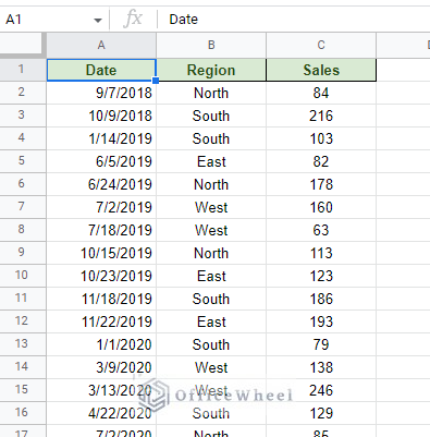
While it is simple to decipher, it is always a good idea to check the validity of the date. We will use the DATEVALUE function for this. Simply apply the formula in a separate cell.
=DATEVALUE(A2)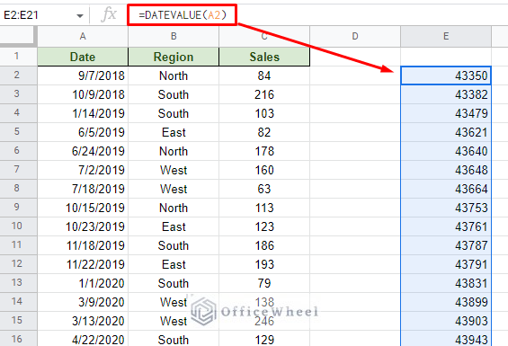
As you can see, all the dates return a numerical value, confirming that these dates are valid.
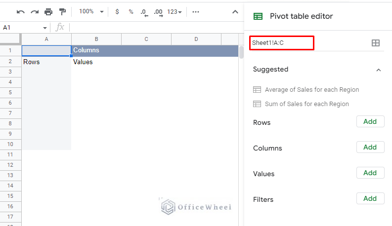
Step 2: Create a pivot table. We will use the current dataset to create the pivot table.
Select entire columns > Insert > Pivot Table > New Sheet
We will get the following pivot table:
Step 3: Add data to the pivot table. The objective is to present the total sales by date.
For the Rows condition, we use Date. And for Values, we use Sales data.
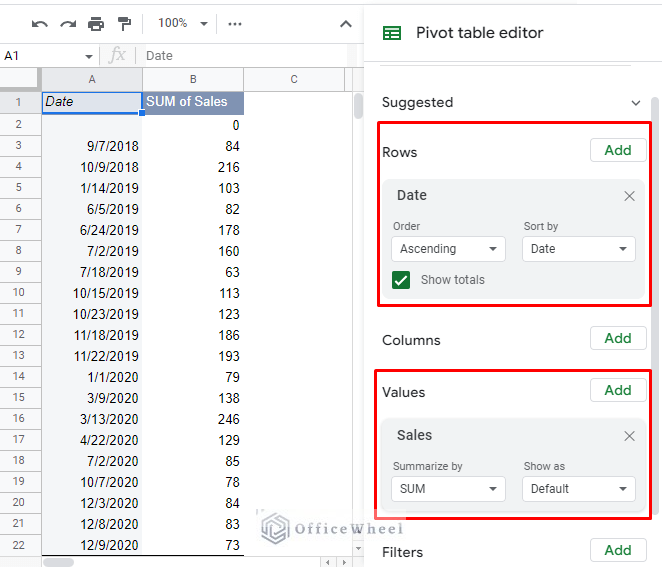
As you can see, there is not much difference between the pivot table and the source dataset. This is why it is so important to further summarize this data by grouping.
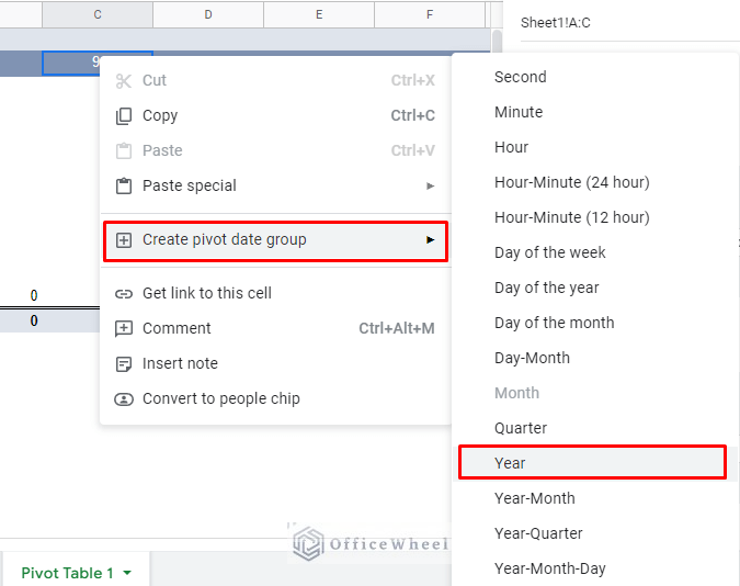
At this point, we have several options to group by date values in the pivot table. Simply right-click over any date to bring up the pivot table group menu:
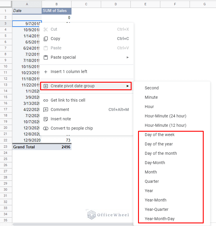
However, we will focus on some of the most commonly used options with some iterations:
- Month
- Month and Year
- Quarter
- Week Number
Let’s see what they look like.
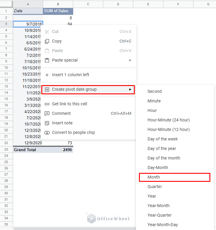
1. Group by Month in a Google Sheets Pivot Table
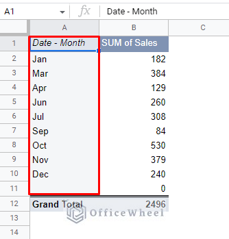
Continuing from where we left off. Right-click on any of the date values on the pivot table to bring up the grouping menu. This time, select the Month option.
What we get is the sum of Sales for each month:
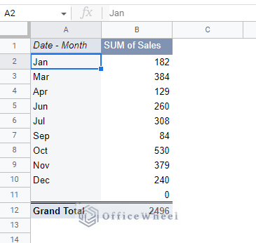
The blank row at the bottom can be ignored as it is accommodating all the blank cells in the source data set range.
One thing to note about this grouping of months is that years are not considered. So, whatever the year, as long as the data fall in a particular month, the data will be grouped accordingly.
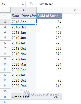
2. Group by Year-Month
The next date group of pivot tables in Google Sheets is the Year-Month group:
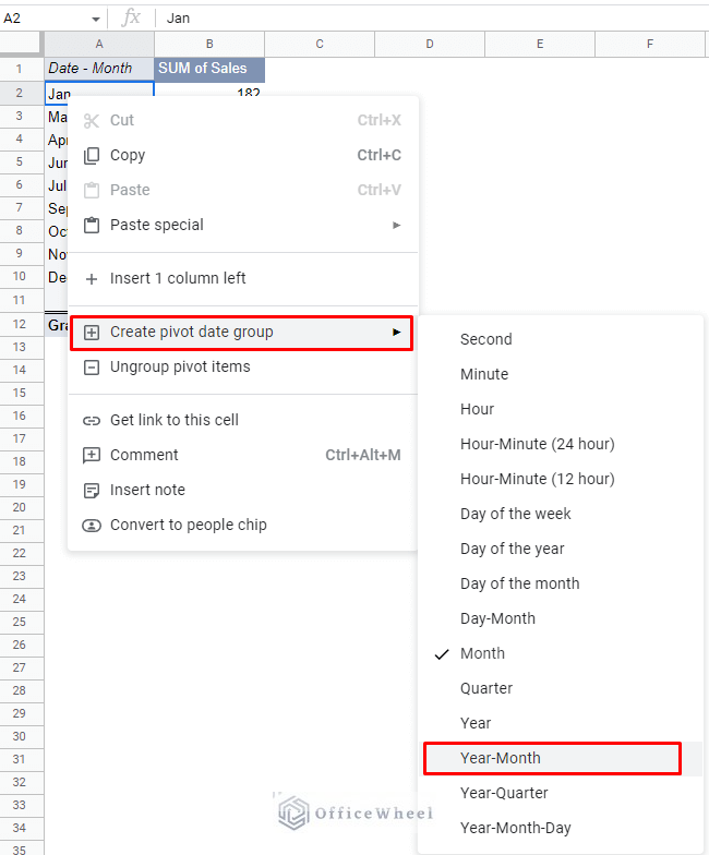
This grouping includes the year that the month is in as well. This adds another layer to the data presented.
Alternative: A Better Representation of Data by Grouping Year and Month Separately
Having the months separated by years is good. But what is better, and frankly, what should be done, is to keep the two sets of groups separate.
What we are looking for is a two-dimensional table with rows having the month group and the years as the columns. Let’s see how it’s done.
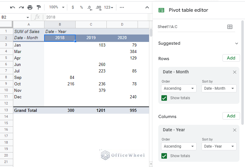
Step 1: Set the primary pivot table column to be grouped by months.
Step 2: Add the Columns value as Date. This will set the two-dimensional layout that we are looking for.
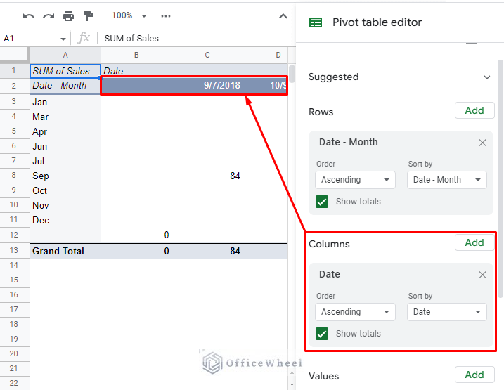
Step 3: This time, we will group the pivot table column as years.
Right-click on any date of the column > Create pivot date group > Year
The result:
3. Quarterly Grouping
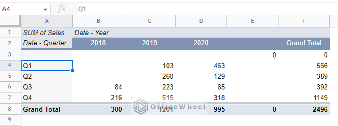
Keeping the columns as years, let’s update the primary column to group the date as yearly quarters.
Right click over any date of the primary column > Create pivot date group > Quarter
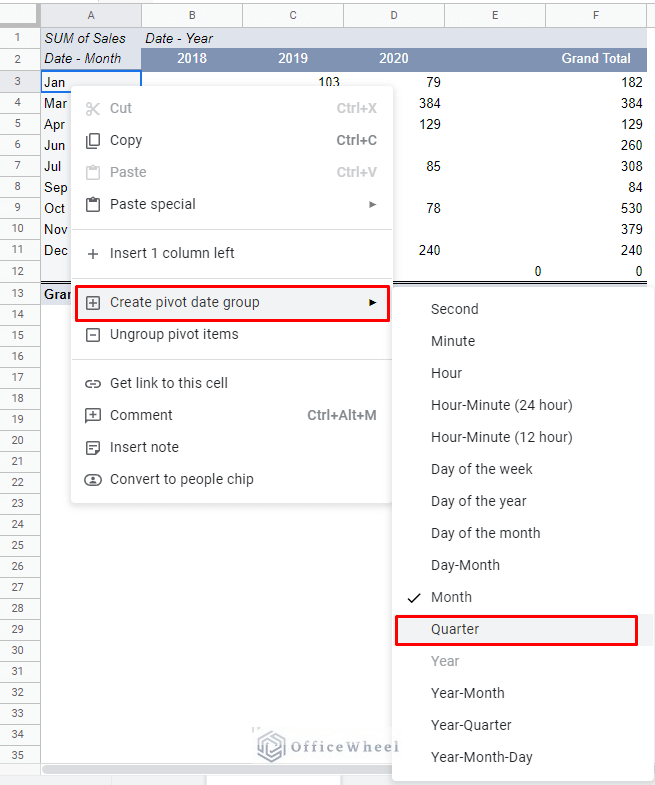
The result:
4. Group by Week Number in a Google Sheets Pivot Table
Occasionally, a user may require the pivot table to group the dates as the week number of the year. This is a rare occurrence, so it is understandable why this grouping option is not available by default.
Thankfully, however, it is not impossible to achieve. We just need a little help, or more precisely, the use of a helper column.
Step 1: Back in the source dataset, create a column called ‘Week No.’. We will apply the WEEKNUM function here with reference to the Date column:
=ArrayFormula(IF(A2:A="","",WEEKNUM(A2:A)))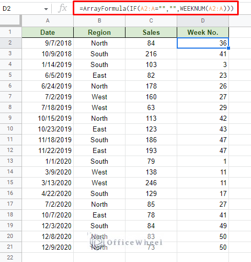
Note: This formula accommodates for black cells (with IF) and any future entries (with an open cell range and ARRAYFORMULA).
Step 2: Update the data range of the pivot table:
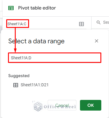
If you are creating a new table altogether, just make sure to include the week number helper column.
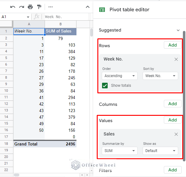
Step 3: Add the ‘Week No.’ condition to Rows. Add ‘Sales’ to Values.
Final Words
Grouping dates in a Google Sheets pivot table is a great way to further summarize data. As we have shown, you can also use grouping to create two-dimensional date pivot tables. Of course, pivot tables do not limit groups to just dates.
Feel free to leave any queries or advice you might have for us in the comments section below.