We use various functions in Google Sheets to make our data look meaningful. Most of the time you need to copy-paste the functions or drag them to apply the formulas in rows or columns. If you want to perform this task in an efficient and fast way, there is a formula that makes all this work simple and easy. The ARRAYFORMULA function allows you to apply the function to numerous rows and columns at once. In this article, we will discuss how to use this ARRAYFORMULA in Google Sheets.
What Is ARRAYFORMULA in Google Sheets?
The ARRAYFORMULA function allows applying a single formula on multiple rows or/and columns in an array at the same time.
The ARRAYFORMULA is a very time-efficient function. It is dynamic, expandable, and can store data in memory. It is primarily used to present a long array of formula results by utilizing only a single cell.
Syntax
The syntax of ARRAYFORMULA is:
ARRAYFORMULA(array_formula)
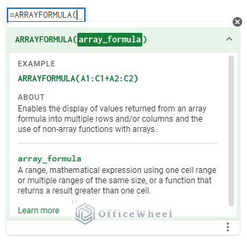
Argument
| ARGUMENT | REQUIREMENT | Function |
|---|---|---|
| array_formula | Required | The argument may consist of a cell range, a function, or a math expression for one or more identical-sized arrays. |
Output
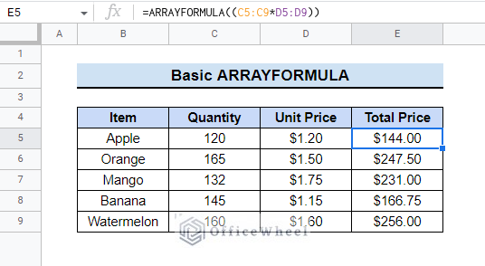
The formula =ARRAYFORMULA((C5:C9*D5:D9)) will show the total price of all the items ranged in cell B5:B9 using the data from cell range C5:C9 and D5:D9.
6 Examples to Use ARRAYFORMULA in Google Sheets
Here we will show some examples to demonstrate how to use ARRAYFORMULA in Google Sheets.
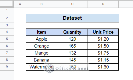
Let’s assume we have a dataset of some items, with their quantity and unit price. We will use ARRAYFORMULA in this dataset to visualize in a more understandable way.
Follow the article and you will be able to apply ARRAYFORMULA by yourself.
1. Applying Basic ARRAYFORMULA Function
Here we will use the ARRAYFORMULA to find out the total price of the items in the dataset. We previously used the regular multiplication and fill handle tool to copy in other cells. On the contrary, now we will use the ARRAYFORMULA that will automatically apply the formula to all cells successively.
📌 Steps:
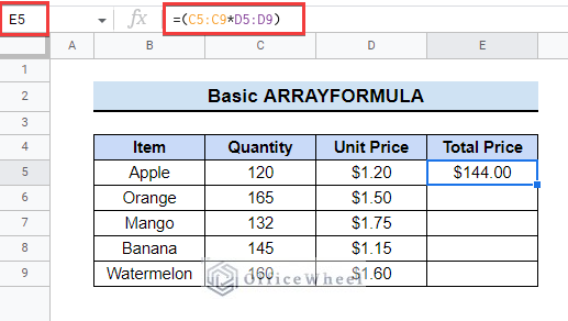
- First, select cell E5 and insert the following formula.
=(C5:C9*D5:D9)
- However, this will only show the first cell of the range multiplied. Although the other results have been calculated, they are not displayed. That’s where ARRAYFORMULA comes in.
- If you want to get the whole range result also, then you have to copy and paste it into other cells or you can apply the below ARRAYFORMULA in cell E5.
=ARRAYFORMULA(C5:C9*D5:D9)
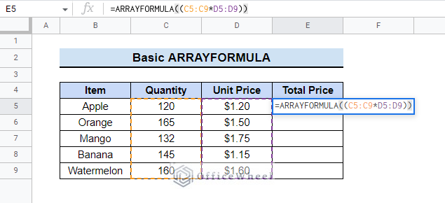
- After that, this formula will result in showing all items’ total prices at once.
Formula Breakdown
- (C5:C9*D5:D9): Here, the formula will give only C5*D5 as output.
- =ARRAYFORMULA(C5:C9*D5:D9): If you put ARRAYFORMULA then it will show results from C5:C9 to C9*D9 successively.
Read More: How to Sum Using ARRAYFORMULA in Google Sheets
2. Combining IF and ARRAYFORMULA Functions
Now we will use the IF function with the ARRAYFORMULA function to apply a condition to sort some data. The IF function returns a value depending on whether it is “TRUE” or “FALSE”.
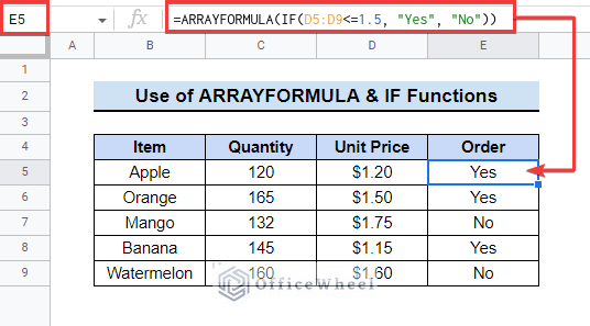
Suppose, you will only order the items whose unit price is below $1.50. So you want to put the decision in another column.
📌 Steps:
- First, select cell E5 and insert the below formula.
=ARRAYFORMULA(IF(D5:D9<=1.5, “Yes”, “No”))
- Then, you will see in the E column the cells will show “Yes” or “No” depending on the unit price.
Formula Breakdown
- (IF(D5:D9<=1.5, “Yes”, “No”): If any value from cell D5 to D9 is below or equal to 1.5, it will return “Yes”, otherwise “No”.
- D5:D9<=1.5: The criterion for the IF function. Checks whether the values in the range D5:D9 is less than or equal to 1.5.
- “Yes”: The result returned if the condition is met.
- “No”: If the value is above 1.5 then the formula will return “No”.
Read More: How to Use ARRAYFORMULA with IF Function in Google Sheets
Similar Readings
- How to Format Date with Formula in Google Sheets (3 Easy Ways)
- Multi Row Dynamic Dependent Drop Down List in Google Sheets
- How to Use RIGHT Function in Google Sheets (6 Suitable Examples)
- How to Use the DATEVALUE Function in Google Sheets (An Easy Guide)
3. Utilizing ARRAYFORMULA with SUMIF Function
We can also utilize ARRAYFORMULA with the SUMIF function. The SUMIF function computes a conditional sum over a range. Follow the steps to do it by yourself.
📌 Steps:
- First, select cell D12 and enter the formula.
=ARRAYFORMULA(SUMIF(B5:B9,C12:C13,E5:E9))
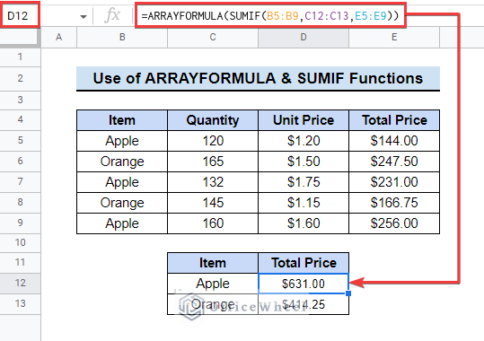
- Then, the formula will automatically show the total price of each item category too.
Formula Breakdown
- B5:B9: This is the SUMIF function criteria range.
- C12:C13: Here, C12 and C13 are the criteria. The function will find the values from the set criteria.
- E5:E9: It is the range for the sum value. The formula will return the sum of each criterion.
Read More: Google Sheets: Sum If there are Multiple Conditions (3 Ways)
4. Applying COUNTIF and ARRAYFORMULA Functions
We often need to find category appearance numbers in a dataset. We use the COUNTIF function to do that. It is hectic to copy-paste the formula into a large dataset. We can use the COUNTIF and ARRAYFORMULA functions together to get values in no time.
📌 Steps:
- First, select cell C13 and enter the below formula.
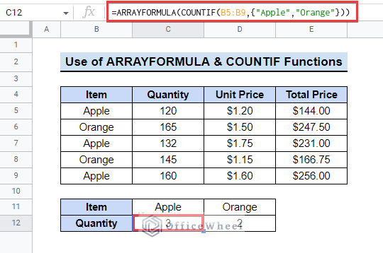
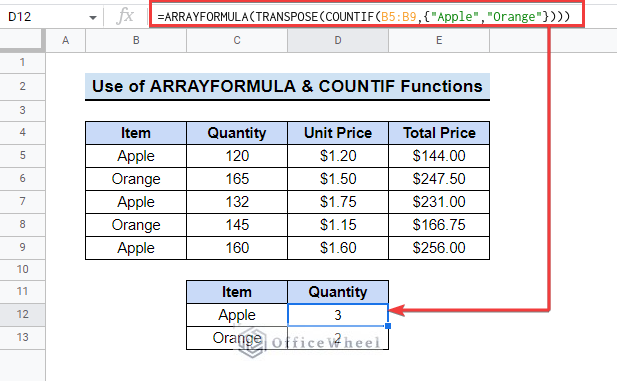
=ARRAYFORMULA(COUNTIF(B5:B9,{"Apple","Orange"}))
- Then, This will show the mentioned items’ appearance number in the dataset with only one formula. Otherwise, you would have to make a COUNTIF formula for each category.
- In this ARRAYFORMULA, you can see that it shows that “Apple” appeared thrice in the dataset and “Orange” twice.
- The COUNTIF with ARRAYFORMULA shows the output horizontally. If you want to see the output vertically then you need to add the TRANSPOSE function in this formula. The TRANSPOSE function flips rows and columns.
- Insert the following formula to get the vertical output like the following image.
=ARRAYFORMULA(TRANSPOSE(COUNTIF(B5:B9,{"Apple","Orange"})))
Formula Breakdown
- B5:B9: This is the COUNTIF function criteria range.
- {“Apple”,”Orange”}: “Apple” and Orange are the criteria. You can add multiple criteria under ARRAYFORMULA.
- (TRANSPOSE(COUNTIF(B5:B9,{“Apple”,”Orange”}))): Here, the TRANSPOSE function changes the orientation of data. It transposes rows and columns.
5. Utilizing VLOOKUP and ARRAYFORMULA Combination
The VLOOKUP function is used to search any data in a table or by row. We can add ARRAYFORMULA to put multiple indexes in the VLOOKUP formula.
📌 Steps:
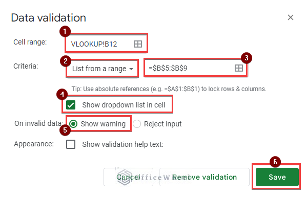
- First, select the cell B12 and make a dropdown of the Item Codes.
- After selecting the cell, go to Data >> Data Validation. And a dialog box will appear.
- Next, select the range and other options just like the following image.
- You can learn how to make a dropdown from here.
- Then, insert the formula in cell C12.
=ARRAYFORMULA(VLOOKUP($B$12,$B$5:$E$9,{2,3,4},FALSE))
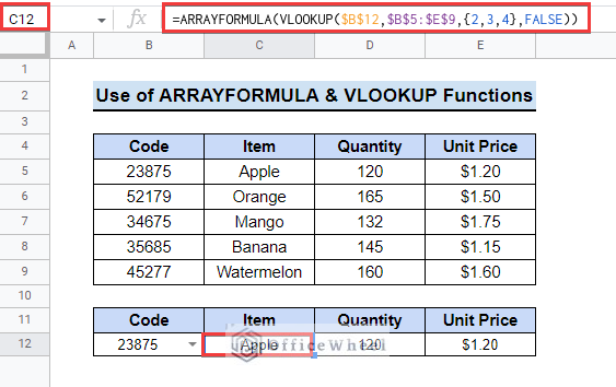
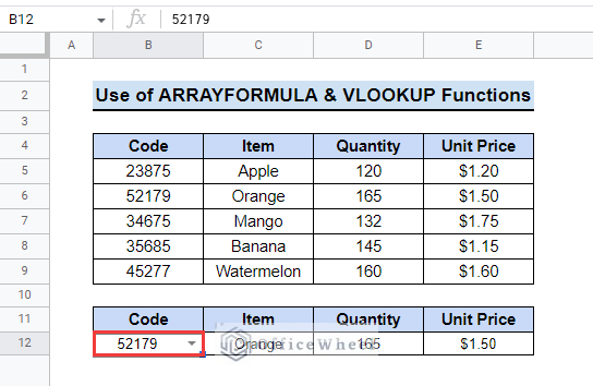
- Now, if you change the dropdown, the VLOOKUP will automatically search for the data.
- Finally, show it in respective columns like the following image.
Formula Breakdown
- $B$12: This $B$12 is the search key, and the function will search data using this input key. Here add the dollar sign to lock the reference. You can use the F4 key to do that or read this article to learn the method.
- $B$5:$E$9: It is the range for the VLOOKUP function.
- 2,3,4: These are the column indexes of the table you want to see as search results.
- False: The term “False” is given to find the exact match from the data table.
Read More: How to Use ARRAYFORMULA with VLOOKUP in Google Sheets
6. Using AVERAGE and ARRAYFORMULA Functions
The AVERAGE function returns the average of a range of numbers. You can use the AVERAGE function within ARRAYFORMULA to get the average of any data without making a new column.
📌 Steps:
- First, select the cell D11 and enter the formula.
=AVERAGE(ARRAYFORMULA((C5:C9*D5:D9)))
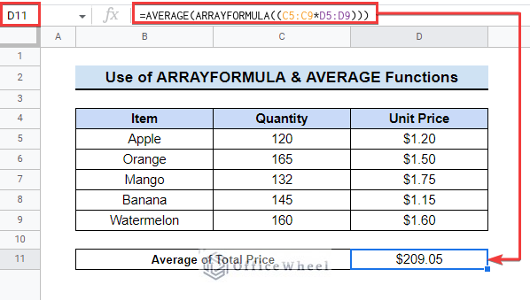
- Then, you can see, the ARRAYFORMULA function contains the formula to get the total price.
- And you can use the AVERAGE function with that to find the total price average without adding a column.
Read More: How to Calculate Weighted Average Using IF Function in Google Sheets
Things to Remember
- You can use the CTRL+SHIFT+ENTER shortcut to add the ARRAYFORMULA function at the beginning of any formula.
- Remember to add the dollar ($) sign in the VLOOKUP formula for fixed reference.
- You cannot export the ARRAYFORMULA function.
Conclusion
Hopefully, the methods above will be enough for you to use ARRAYFORMULA in Google Sheets. You can check the practice spreadsheet and then practice on your own. Please use the comment section below for any further queries or suggestions. You may also visit our OfficeWheel blog to explore more about Google Sheets.
Related Articles
- How to Link Cells Between Tabs in Google Sheets (2 Examples)
- How to Use IF and OR Formula in Google Sheets (2 Examples)
- Google Sheets Use Filter to Remove Duplicates in Column
- Google Sheets: How to Autofill Based on Another Field (4 Easy Ways)
- How to VLOOKUP Last Match in Google Sheets (5 Simple Ways)
- How to Ignore 0 for Standard Deviation Formula in Google Sheets
- 2 Helpful Examples to VLOOKUP by Date in Google Sheets