How to Use Nested VLOOKUP in Google Sheets

Nested VLOOKUP is a powerful technique in Google Sheets that allows you to retrieve data from multiple sources and columns using multiple VLOOKUP functions within a single formula. For example, you can use nested VLOOKUP to find sales data or compare product performance. It not only saves time but also improves accuracy.

A Sample of Practice Spreadsheet

You can copy our spreadsheet that we’ve used to prepare this article.

2 Simple Ways to Use Nested VLOOKUP in Google Sheets

Nested VLOOKUP in Google Sheets enables professionals to quickly retrieve and analyze large amounts of data from multiple tables or sheets. By allowing users to easily access and compare relevant information from various sources. There are two types of use of nested VLOOKUP in Google Sheets.

1. Using Single Criteria

Nested VLOOKUP with a single criterion is a variant of the VLOOKUP function in Google Sheets that allows you to search for a specific value in a range of cells and retrieve a corresponding value from a different column.
We will use the following data for example to describe the whole process.

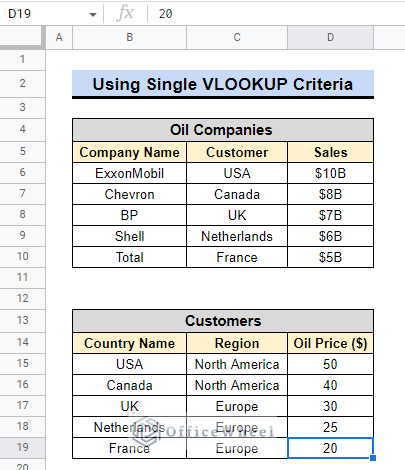
Imagine we have two different datasets containing information about oil companies, their customers, and sales. Using a nested VLOOKUP with a single criteria, we can determine where Chevron is exporting its products.

Steps:

• To find the export region of Chevron oil company, start by selecting cell G6.

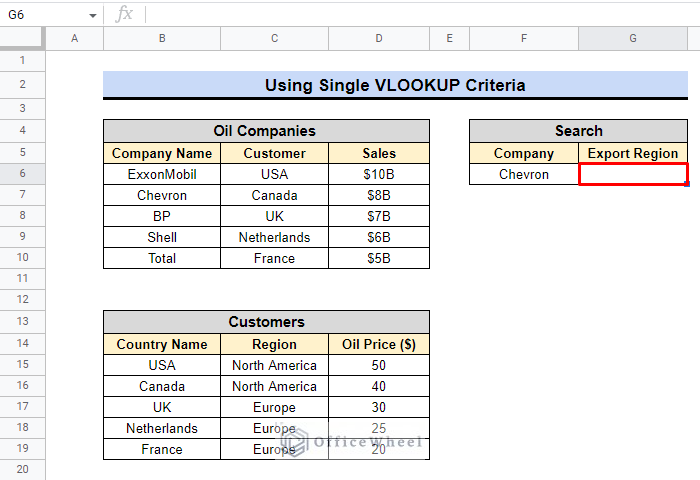
• Then, we will use the formula:

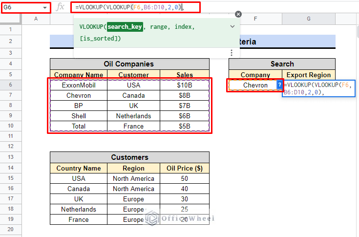
• The latter VLOOKUP function searches for the value in cell F6 (which is “Chevron“) in the range B6:D10 in table 1.
• The return value by the latter VLOOKUP is Canada which will be the search key for the former VLOOKUP.

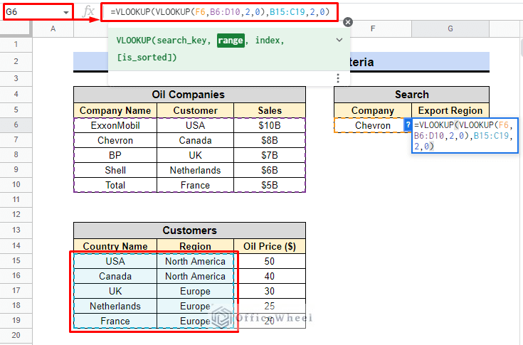
• The final formula is:

• The former VLOOKUP function then searches for the resulting value (which is “North America“) in the range B16:C20 in table 2.
• The third argument for both VLOOKUP functions is 2, which tells the function to return the second column in the specified range.
• The fourth argument for both VLOOKUP functions is 0, which tells the function to find an exact match.

• Press ENTER to see the result.

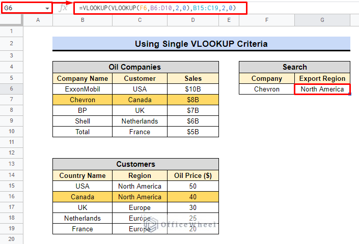
The nested VLOOKUP function has successfully identified that Chevron primarily sells its oil in Canada, which is located in North America, as shown in the image above.

Read More: Alternative to Use VLOOKUP Function in Google Sheets

A Different Approach: Reverse Nested VLOOKUP

Reverse Nested VLOOKUP is a variation of the traditional Nested VLOOKUP function, where the lookup value is on the right side of the table instead of the left. This function is useful in cases where the lookup value is dynamic and the table data is fixed, allowing for a more flexible and efficient data analysis process.

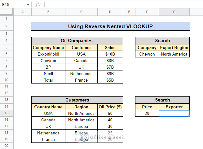
In this scenario, we will use the reverse nested VLOOKUP formula to find the company that sells oil at the lowest price using the same dataset.

Steps:

• First, we’ll choose cell G15.
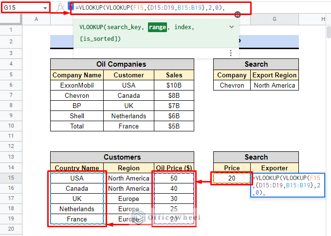
• Afterward, we’ll apply the following formula.

• The inner VLOOKUP searches for the cell value of F16 in the range sequentially {D16:D20,B16:B20} and returns the value from the second column (column index 2).
• The 0 at the end of the inner VLOOKUP function specifies that an exact match is required.

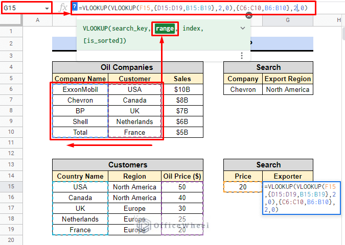
• The final formula is as follows.

• The outer VLOOKUP uses the result from the inner VLOOKUP as the search key and searches for it in the range {C6:C10,B6:B10} in a specified order.
• The outer VLOOKUP returns the value from the second column (column index 2) of the range {C6:C10,B6:B10} where the search key is found.

• Once again, press ENTER to view the outcome.

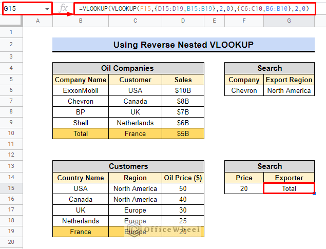
From the above image, we may infer that the reverse nested VLOOKUP function was able to look up the value 20 in a different way than in a conventional way, and as a result, we learn that Total Company offers oil for the lowest price.

Read More: How to Do Reverse VLOOKUP in Google Sheets (4 Useful Ways)

Similar Readings

• Create Hyperlink to VLOOKUP Cell in Multiple Rows in Google Sheets
• VLOOKUP with IMPORTRANGE Function in Google Sheets
• How to Use VLOOKUP with Named Range in Google Sheets
• VLOOKUP Last Match in Google Sheets (5 Simple Ways)
• How to Use VLOOKUP for Conditional Formatting in Google Sheets

2. Applying Multiple Criteria

Professionals often use multiple criteria in VLOOKUP to improve the accuracy and efficiency of their data analysis. We’ll go over a few instances to show how to use multiple criteria with VLOOKUP.

I. Using Ampersand to Join Multiple Criteria in VLOOKUP

Consider two independent datasets containing information about oil companies, their customers, and their sales.

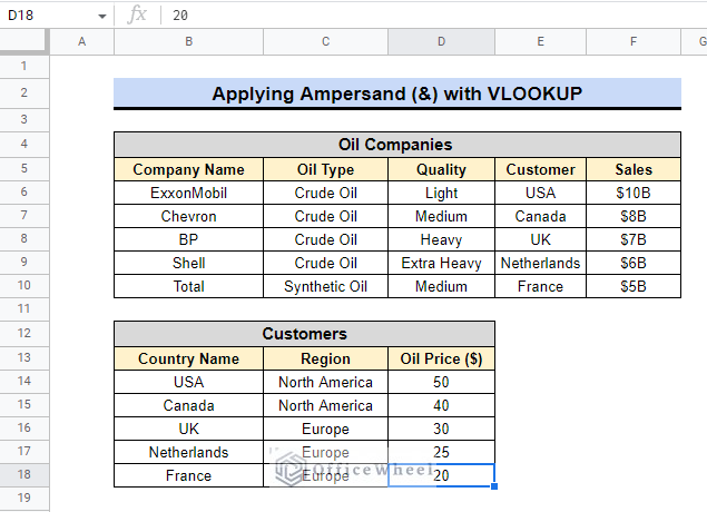
Consider the situation where we need to locate a company that supplies medium quality crude oil. The steps below will help us find the solution.

Steps:

• Firstly, we’ll create a Helper Column and link the two columns D and E.
• We must maintain this Helper Column in the first position since the VLOOKUP function searches for a value in the first column.
• Secondly, in cell B6, we’ll apply the following formula.

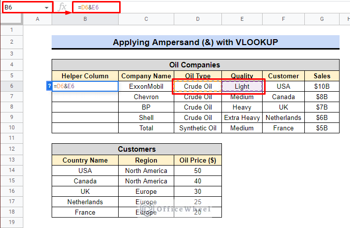
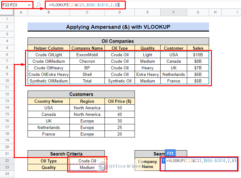
• Furthermore, to start the search, we will now choose cell F22.
• We will later use the formula below to pinpoint the appropriate company.

• To view the outcome, press ENTER at the very end.

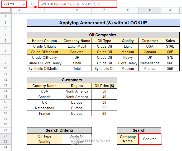
Therefore, using Ampersand (&) with the VLOOKUP function to search for a value in a table and then return a value from a certain column in that table is successful. Since We ultimately discovered that Chevron offers crude oil that is of medium quality.

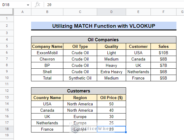
II. VLOOKUP with MATCH Function

We’ll use the same dataset as previously, but this time we’ll search for a company that offers oils for sale in the Netherlands for $25. Check out the next few steps to learn how to use VLOOKUP with the MATCH function when there are multiple criteria.

Steps:

• Once again we need the help of Helper Column similarly to link the Country name and the Oil Price.
• In addition, we will use the following formula to merge or join them.

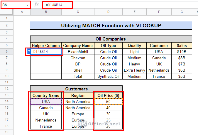
• Afterward, we will select cell F22.
• We will use the following formula to find the Company that distributes oil in the Netherlands.

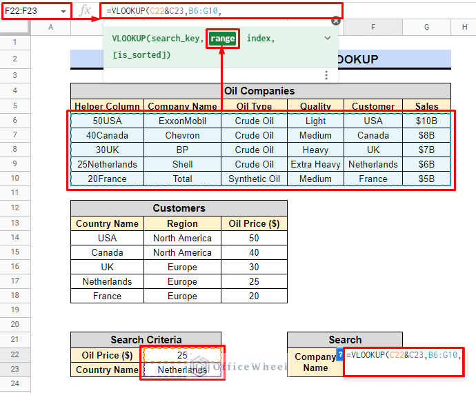
• C22&C23 is the search value. The & operator combines the values in cells C22 and C23 into a single string.
• B6:G10 is the range that we are searching in. This is the table that contains the data we are interested in.
• To use the MATCH function as the column index in VLOOKUP, we will use the following formula.

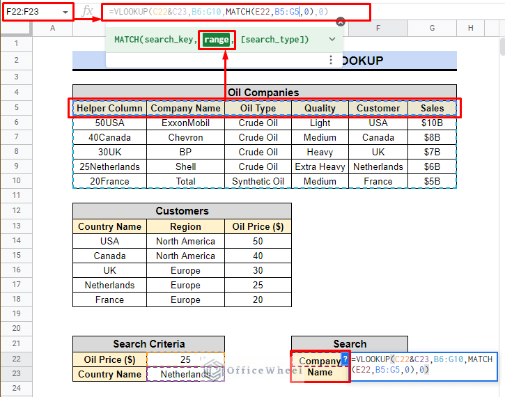
• The MATCH function looks for the value of cell E22 in the range B5:G5, and returns the index of the column.
• 0 is the optional fourth argument for the VLOOKUP function, which specifies that we want an exact match.

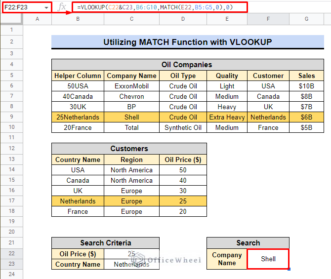
According to the aforementioned image, we find that Shell is the primary oil distributor in the Netherlands and charges $25 per barrel.

Read More: How to VLOOKUP All Matches in Google Sheets (2 Approaches)

Conclusion

The nested VLOOKUP function in Google Sheets enables users to search for specific data within multiple columns and return the desired result. It is useful for professionals dealing with large datasets and needing to efficiently retrieve and analyze data. Check out the website, OfficeWheel, for help in professional work.

Related Articles

• Google Sheets Vlookup Dynamic Range
• How to Use Wildcard in Google Sheets (3 Practical Examples)
• Check If Value Exists in Range in Google Sheets (4 Ways)
• [Fixed!] Google Sheets If VLOOKUP Not Found (3 Suitable Solutions)
• VLOOKUP Error in Google Sheets (with Quick Solutions)
• How to VLOOKUP Multiple Columns in Google Sheets (3 Ways)
• [Solved!] VLOOKUP Function Is Not Working in Google Sheets
• How to Use VLOOKUP Function for Exact Match in Google Sheets