We normally use the IF function to logically match some values in Google Sheets. But sometimes the given dataset is huge and then it is boring to use the same formula again and again. We can solve this issue by using the ARRAYFORMULA function. This function enables us to expand the result through the whole dataset with a single click. In this article, I’ll show you 3 quick examples to use the ARRAYFORMULA with the IF Function in Google Sheets.
A Sample of Practice Spreadsheet
You can download Google Sheets from here and practice very quickly.
3 Suitable Examples to Use ARRAYFORMULA with IF Function in Google Sheets
Let’s get introduced to our dataset first. Here we have some products in Column B and their sales price in Column C. With the help of this dataset, I’ll show you 3 practical examples to use the ARRAYFORMULA with the IF function in Google Sheets.
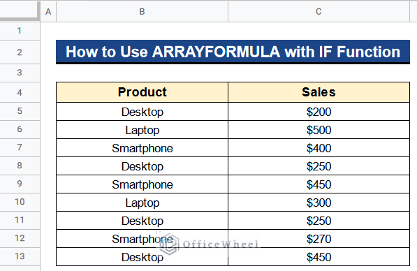
Example 1. Combining ARRAYFORMULA with IF Function
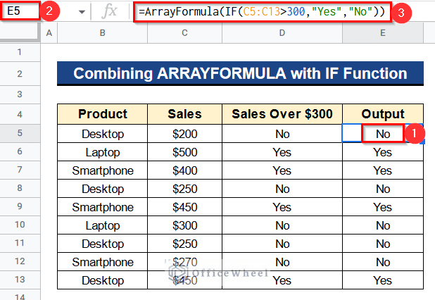
Foremost we can combine the ARRAYFORMULA with the IF function to calculate something very fast without repeating the process. Like here in our dataset we want to get output as Yes if the sales price is greater than $300 otherwise No. We can do it simply by the IF function. But it’ll take a lot of time. So we’ll do it by combining the ARRAYFORMULA with the IF Function. First, I’ll show the process by the IF function. Then I’ll do it by our desired method.
Steps:
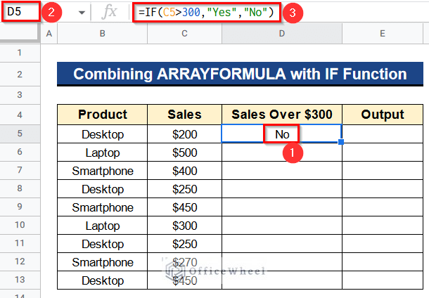
- Firstly, type the following formula in Cell D5-
=IF(C5>300,"Yes","No")- Then hit Enter to get the output.
- Secondly, apply the Fill Handle tool to use the formula in all columns.
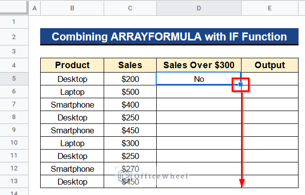
- Lastly, you’ll get your desired result. But this process is taking so much time. So we’ll use the combination of the ARRAYFORMULA with the IF function now.
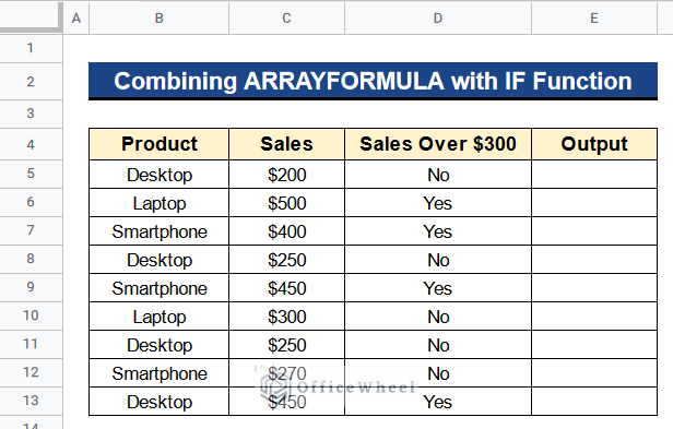
- At first, insert the following formula in Cell E5-
=ARRAYFORMULA(IF(C5:C13>300,"Yes","No"))- Finally, press Enter to get all the results at once, and no need of using the Fill Handle tool.
Formula Breakdown
- IF(C5:C13>300,”Yes”,”No”)
At first, this function will search for sales values greater than $300 from Cells C5 to C13 and returns Yes if the condition is true. Otherwise, it returns No.
- ArrayFormula(IF(C5:C13>300,”Yes”,”No”))
Finally, this function expands the result over the full range and gives results directly as an array.
Read More: How to Sum Using ARRAYFORMULA in Google Sheets
Example 2. Joining ARRAYFORMULA with IF, LEN, VLOOKUP, and QUERY Functions
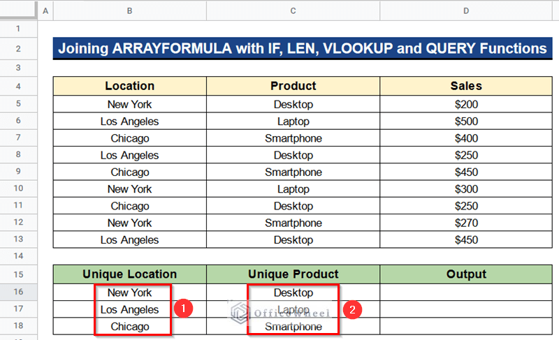
Now we have a different dataset as shown in the picture. We have different locations in Column B, different products in Column C, and their sales price in Column D. Moreover, we have some unique locations and products in different places below Column B and Column C. At present we want sales price based on these 2 criteria. For that purpose, we can use the combination of the ARRAYFORMULA with IF, LEN, VLOOKUP, and QUERY functions. Let’s see how to do that.
Steps:
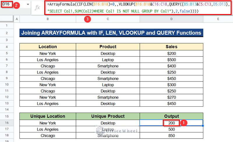
- Foremost, write the following formula in Cell D16-
=ARRAYFORMULA((IF(LEN(B16:B18)=0,,VLOOKUP(B16:B18&C16:C18,QUERY({B5:B13&C5:C13,D5:D13}, "SELECT Col1,SUM(Col2)WHERE Col1 IS NOT NULL GROUP BY Col1"),2,False)))- At last, press Enter Button to get the output.
Formula Breakdown
- LEN(B16:B18)
Firstly, this function searches for the length of the values from Cell B16 to B18 which have unique locations.
- QUERY({B5:B13&C5:C13,D5:D13}
It queries the values in Column B and Column C that have locations and products. After that, it queries their sales price.
- VLOOKUP(B16:B18&C16:C18,QUERY({B5:B13&C5:C13,D5:D13}, “SELECT Col1,SUM(Col2)WHERE Col1 IS NOT NULL GROUP BY Col1”)
From Cell B16 to B18 we have unique locations and from Cell C16 to C18 we have unique products. Now the VLOOKUP function will search for these values with the help of the QUERY function and give the value of the sales price.
- IF(LEN(B16:B18)=0,,VLOOKUP(B16:B18&C16:C18,QUERY({B5:B13&C5:C13,D5:D13}, “SELECT Col1,SUM(Col2)WHERE Col1 IS NOT NULL GROUP BY Col1”),2,False)
Next, this function will search for the sales price in Column C by matching it with Column B and give the exact result.
- ARRAYFORMULA((IF(LEN(B16:B18)=0,,VLOOKUP(B16:B18&C16:C18,QUERY({B5:B13&C5:C13,D5:D13}, “SELECT Col1,SUM(Col2)WHERE Col1 IS NOT NULL GROUP BY Col1”),2,False)))
In the end, this function expands the result over all columns and rows as an array.
Read More: How to VLOOKUP Multiple Columns in Google Sheets (3 Ways)
Example 3. Uniting ARRAYFORMULA with IF Function for Multiple Conditions
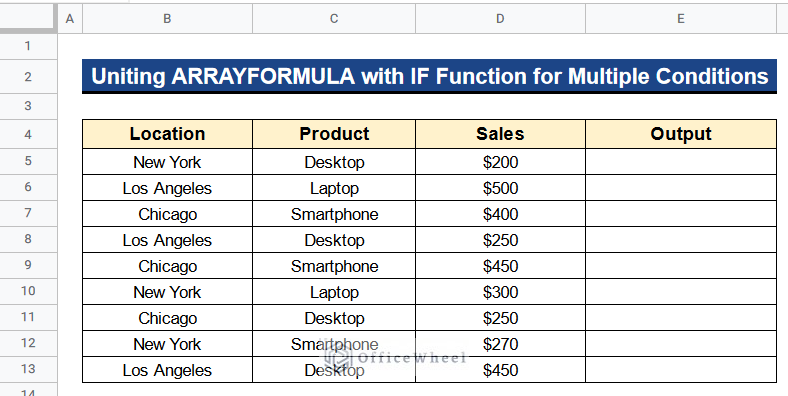
Let’s look into another problem. We have the same dataset as example 2. Now we want Yes or No as output based on matching values from Columns B, C, and D. These things fall into multiple conditions category. As a result, we can unite the ARRAYFORMULA with the IF function to solve the issue.
Steps:
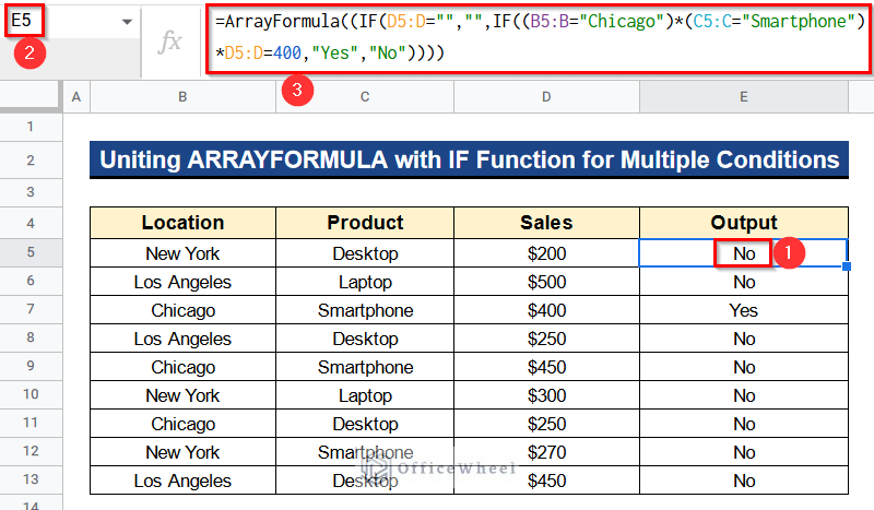
- In the beginning, insert the following formula in Cell E5-
=ARRAYFORMULA((IF(D5:D="","",IF((B5:B="Chicago")*(C5:C="Smartphone") *D5:D=400,"Yes","No"))))- Then, hit Enter to get the desired output as shown in the picture.
Formula Breakdown
- IF(D5:D=””,””,IF((B5:B=”Chicago”)*(C5:C=”Smartphone”) *D5:D=400,”Yes”,”No”))
At first, this function search for Chicago in Column B, Smartphone in Column C, and 400 in Column D. Then it returns Yes or No based on matching.
- ARRAYFORMULA((IF(D5:D=””,””,IF((B5:B=”Chicago”)*(C5:C=”Smartphone”) *D5:D=400,”Yes”,”No”))))
Finally, this function makes an array and gives results quickly.
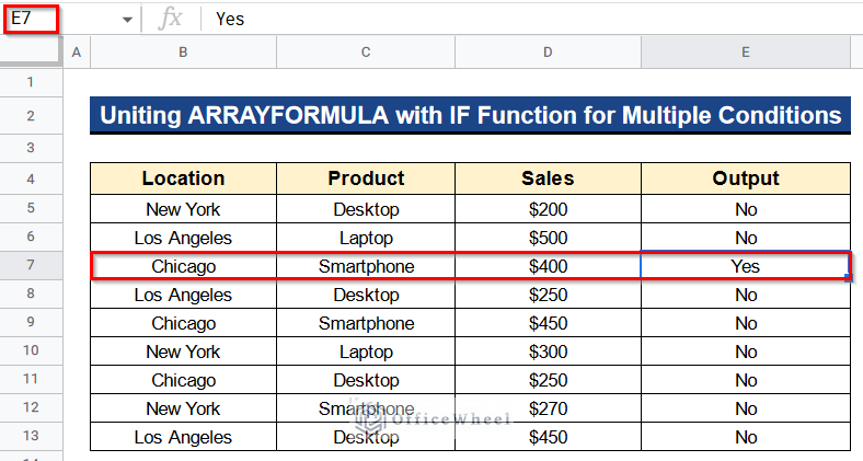
- Finally, you’ll notice that only Row 7 satisfies the given condition. So the output in Cell E7 is Yes.
Read More: Google Sheets: Conditional Formatting with Multiple Conditions
Similar Readings
- How to Do IF THEN in Google Sheets (3 Ideal Examples)
- VLOOKUP with Multiple Criteria in Google Sheets
- How to Use Nested IF Function in Google Sheets (4 Helpful Ways)
- Use VLOOKUP for Conditional Formatting in Google Sheets
- How to Use RIGHT Function in Google Sheets (6 Suitable Examples)
What to Do When ARRAYFORMULA with IF Function Is Not Working?
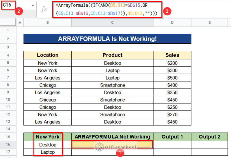
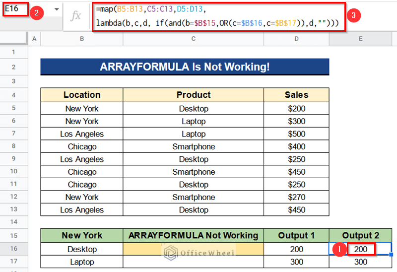
Sometimes you might find that the combination of the ARRAYFORMULA with the IF function is not working. Like in our case we have a fixed location now, which is New York. Now we want to get the sales price of Desktop and Laptop based on the location, New York. So we use the combination of ARRAYFORMULA with IF, AND, and OR functions but the formula isn’t working as we can see in the picture. If we use the IF, AND, and OR functions together it’ll work nicely. But the combination of ARRAYFORMULA with IF, AND, and OR functions don’t work in Google Sheets. That is why we have to use a separate method. We have put the following formula in Cell C16–
=ArrayFormula((IF(AND(B5:B13=$B$15,OR (C5:C13=$B$16,C5:C13=$B$17)),D5:D13,"")))As we can see in the picture the above formula isn’t working. We can resolve this issue by uniting the ARRAYFORMULA with the IF Function. Moreover, we can use the combination of the MAP, LAMBDA, IF, AND, OR functions instead of ARRAYFORMULA to solve the issue. We have shown it below.
Steps:
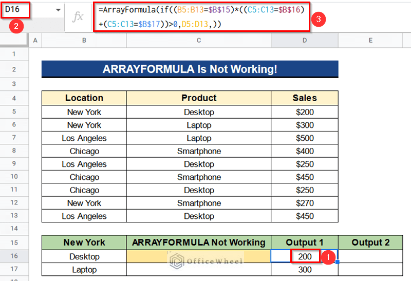
- Before all, insert the following formula in Cell D16-
=ARRAYFORMULA(IF((B5:B13=$B$15)*((C5:C13=$B$16)+(C5:C13=$B$17))>0,D5:D13,))- Then, press Enter to get the result at once.
Formula Breakdown
- IF((B5:B13=$B$15)*((C5:C13=$B$16)+(C5:C13=$B$17))>0,D5:D13,)
Foremost this function searches for location in Column B and products in Column C. Next, it gives the corresponding sales price which is in Column D.
- ARRAYFORMULA(IF((B5:B13=$B$15)*((C5:C13=$B$16)+(C5:C13=$B$17))>0,D5:D13,))
In the end, this formula expands it to the whole output range.
- We can also use another formula other than the ARRAYFORMULA.
- In the first place, type the following formula in Cell E16-
=MAP(B5:B13,C5:C13,D5:D13,LAMBDA(b,c,d,IF(AND(b=$B$15,OR(c=$B$16,c=$B$17)),d,"")))- Then, press Enter Button to get the result quickly.
Formula Breakdown
- OR(c=$B$16,c=$B$17)
At first, this function searches for the values from Cell B16 and Cell B17 in the dataset.
- AND(b=$B$15,OR(c=$B$16,c=$B$17))
Then this formula searches for the value from Cell B15 and gives results based on the previous searches by the OR function.
- IF(AND(b=$B$15,OR(c=$B$16,c=$B$17)),d,””)
Again this function logically searches for the given values from Cell B15, B16, and B17 and gives true if it logically matches the criteria.
- LAMBDA(b,c,d,IF(AND(b=$B$15,OR(c=$B$16,c=$B$17)),d,””))
This formula creates a custom function based on our criteria. In this case, our criteria are locations and products.
- MAP(B5:B13,C5:C13,D5:D13,LAMBDA(b,c,d,IF(AND(b=$B$15,OR(c=$B$16,c=$B$17)),d,””)))
Finally, this function will map each value through the whole dataset based on the LAMBDA function and gives the output like an array.
Read More: How to Use IF and OR Formula in Google Sheets (2 Examples)
Conclusion
That’s all for now. Thank you for reading this article. In this article, I have discussed how to use the ARRAYFORMULA with the IF function in Google Sheets. I have also discussed what to do when ARRAYFORMULA with the IF function is not working in Google Sheets. Please comment in the comment section if you have any queries about this article. You will also find different articles related to google sheets on our officewheel.com. Visit the site and explore more.
Related Articles
- How to Use IF Condition Between Two Numbers in Google Sheets
- Use REGEXMATCH Function for Multiple Criteria in Google Sheets
- Match Multiple Values in Google Sheets (An Easy Guide)
- How to Create Dependent Drop Down List in Google Sheets
- Use Formula to Highlight Duplicates in Google Sheets
- Conditional Formatting with Multiple Conditions Using Custom Formulas in Google Sheets
- Use Multiple IF Statements in Google Sheets (5 Examples)
- Google Sheets: Sum of Cells with Text (4 Examples)