When a dataset has duplicate quantities, you may wish to highlight those duplicates to visualize the dataset. You may wish to highlight those duplicates in various ways each time. In this post, we’ll show you how to use a formula to highlight duplicates in Google Sheets in six different ways.
6 Examples of Using Formula to Highlight Duplicates in Google Sheets
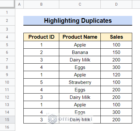
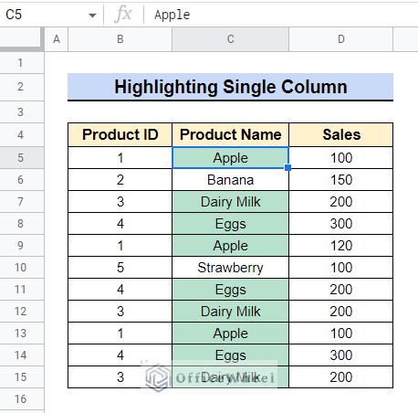
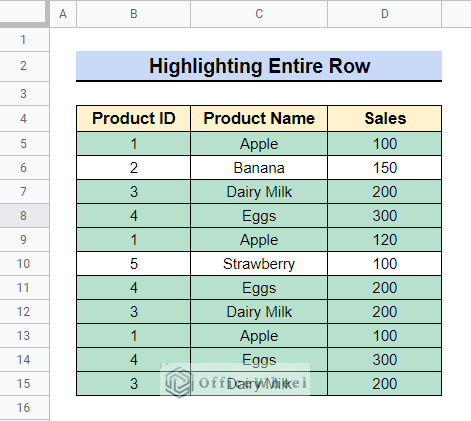
The dataset below will be used to demonstrate examples of how to use a formula to highlight duplicates in Google Sheets. This dataset contains the product id, product name, and product sales of a shop on a particular day. We will highlight the duplicates of this dataset in Google Sheets. Basically, we will use a formula in Conditional Formatting to highlight duplicates in Google Sheets.
1. Highlight Duplicates in a Single Column
One of the most popular Google Sheets features is highlighting duplicates in a single column. We can quickly identify duplicates in a single column using the Conditional Formatting tools in Google Sheets. We will use the COUNTIF function in it to highlight the duplicates.
Steps:
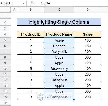
- Select the data range from which you want to highlight the duplicates. We chose Cell C5:C15.
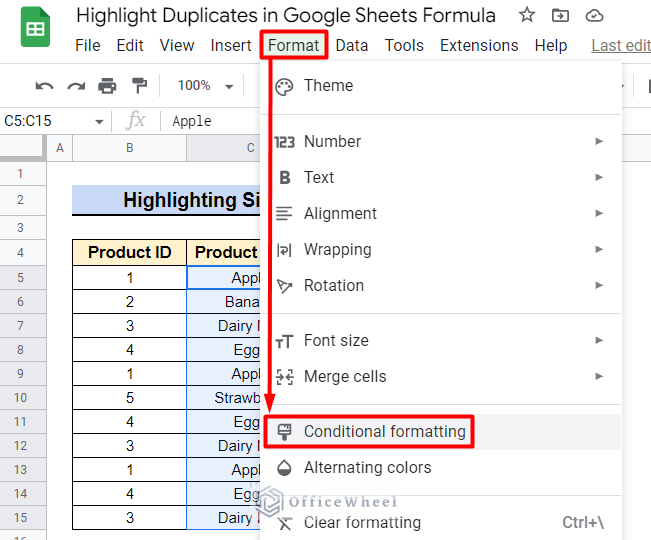
- Go to the Format bar from the top menu bar and select Conditional formatting.
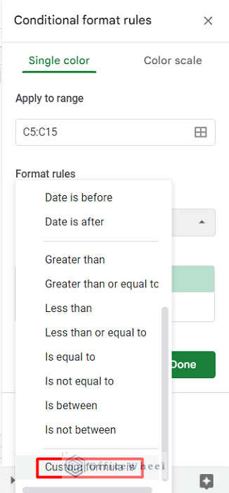
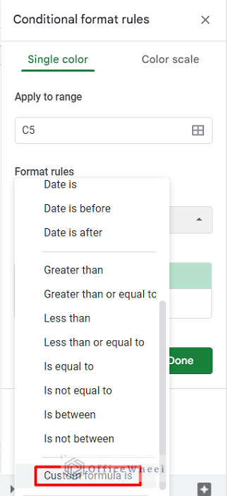
- The Conditional format rules dialog box will open. Now click on the drop-down icon bar in the Format cells if…. option.
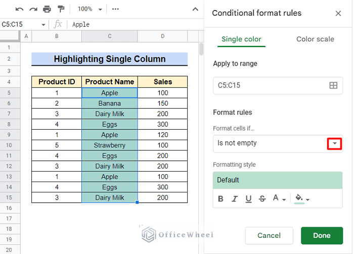
- Choose Custom formula is from the Format cells if…. option.
- Type the formula in the Formula bar option and click Done.
=COUNTIF($C$5:$C$15,$C5)>1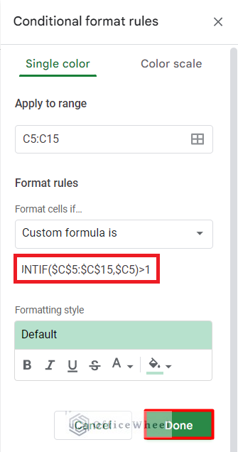
- All the duplicates in the Product Name column are highlighted.
Read More: How to Merge Columns in Google Sheets
2. Insert Formula to Highlight Duplicates in Multiple Columns
Your dataset in Google Sheets can have duplicate values in several columns. Importantly, Google Sheets allows you to use a single formula to indicate duplicates across multiple columns. We will use the same COUNTIF function in a different way to highlight the duplicates.
Steps:
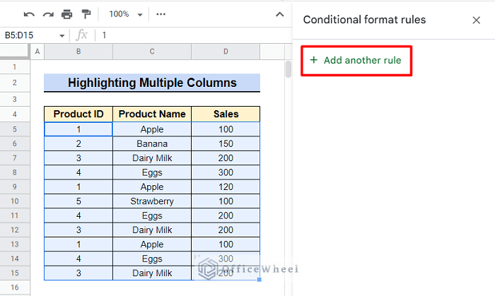
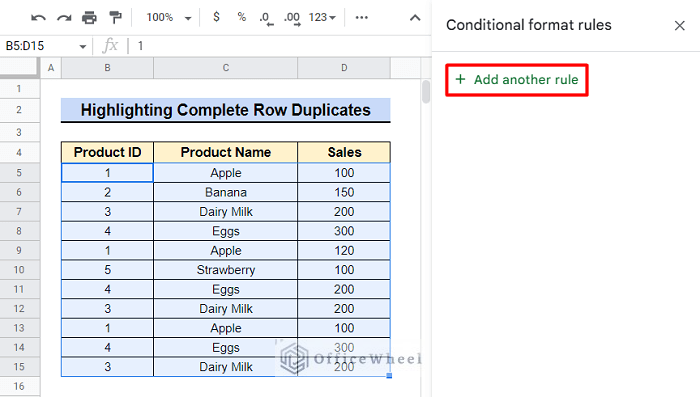
- Choose the data range where you want to highlight the duplicates. We chose Cell B5:D15. Select Add another rule from the Conditional format rules dialog box.
- As mentioned before, click on the drop-down icon bar in the Format cells if…. option and choose Custom formula is.
- Now type the formula in the Formula bar option and click Done.
=COUNTIF($B$5:$D$15,B5)>1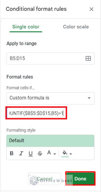
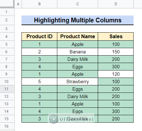
- All the duplicates from multiple columns are now highlighted.
Read More: How to Highlight Duplicates for Multiple Columns in Google Sheets
3. Ignore the First Instance to Highlight Duplicates
In Google Sheets, you might want to ignore the first duplicate and highlight the others as you might wish to get rid of the others later. We will use the same COUNTIF function again to highlight the duplicates.
Steps:
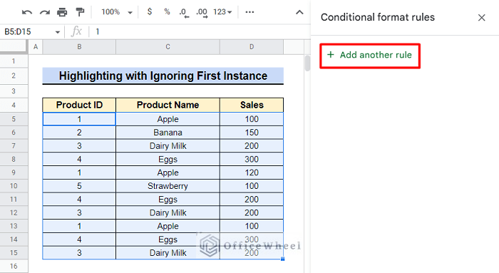
- Choose the data range to highlight duplicates. We chose Cell B5:D15. From the Conditional format rules dialog box, select Add another rule.
- After completing the steps previously mentioned, enter the formula below in the Formula bar option and click Done.
=COUNTIF($B$5:$B5,$B5)>1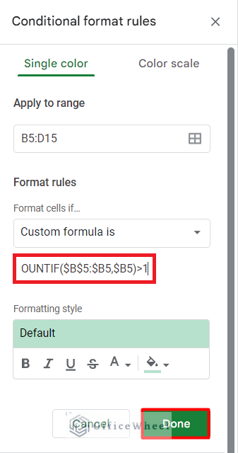
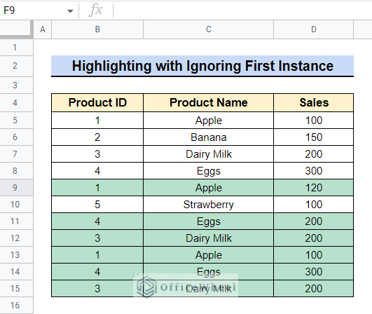
- All the duplicates ignoring the first instance are now highlighted.
Similar Readings
- How to VLOOKUP Last Match in Google Sheets (5 Simple Ways)
- Multi Row Dynamic Dependent Drop Down List in Google Sheets
- How to VLOOKUP with Multiple Criteria in Google Sheets
- Google Sheets: How to Autofill Based on Another Field (4 Easy Ways)
- Sort a Pivot Table in Google Sheets (An Easy Guide)
4. Highlight the Entire Row If Duplicates Are in One Column
If you have duplicates in a particular column, you may occasionally wish to highlight the entire row to visualize the dataset in Google Sheets. Here we’ll highlight the entire row based on Column C and again we’ll use the COUNTIF function to highlight the duplicates.
Steps:
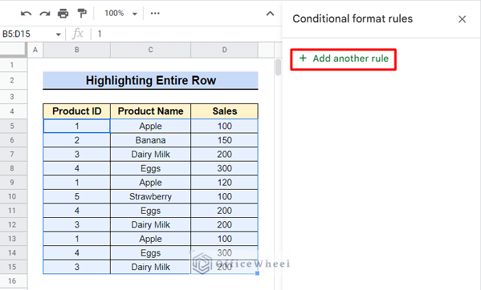
- To highlight duplicates, choose the data range. We chose Cell B5:D15. Select Add another rule from the Conditional format rules dialog box.
- After completing the aforementioned steps, type the following formula into the Formula bar option, then click Done.
=COUNTIF($C$5:$C15,$C5)>1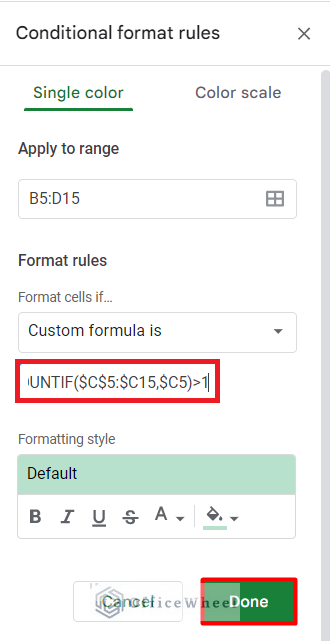
- All rows that contain duplicates in the Product Name column are now highlighted.
Read More: How to Sum Multiple Rows in Google Sheets (3 Ways)
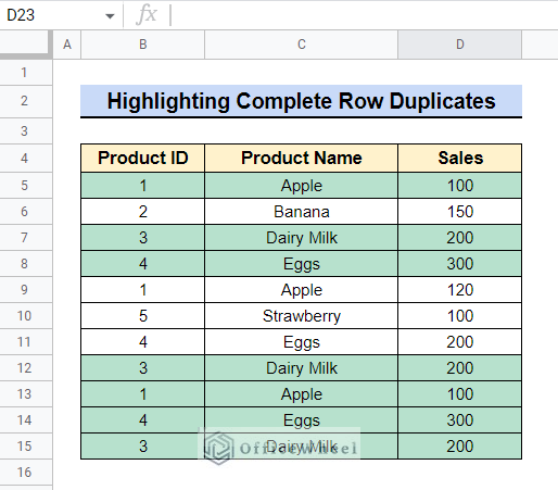
5. Apply Formula to Highlight Complete Row with Duplicates
In Google Sheets, sometimes you may wish to highlight the row if every column in the dataset is an exact match. To accomplish this, before utilizing the COUNTIF function, we need to use the ARRAYFORMULA function to consolidate the data into a single string.
Steps:
- To highlight duplicates, select the data range. We selected Cell B5:D15. Select Add another rule from the Conditional format rules dialog box.
- After completing the previously mentioned steps, type the below formula into the Formula bar option, then click Done.
=COUNTIF(ARRAYFORMULA($B$5:$B$15&$C$5:$C$15&$D$5:$D$15),$B5&$C5&$D5)>1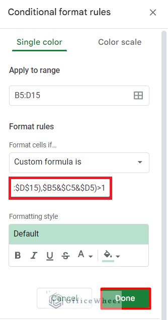
Formula Breakdown:
- ARRAYFORMULA($B$5:$B$15&$C$5:$C$15&$D$5:$D$15)
First, the ARRAYFORMULA function will generate an array of strings by combining the contents of each row’s cells.
- COUNTIF(ARRAYFORMULA($B$5:$B$15&$C$5:$C$15&$D$5:$D$15),$B5&$C5&$D5)>1
Then, the COUNTIF function will use the ARRAYFORMULA as a range and it will count the number of times the combined string appears in the array. If it appears more than 1 time, it will highlight the combined string.
- All of the complete row duplicates are now highlighted.
 Read More: How to Sum Using ARRAYFORMULA in Google Sheets
6. Use Added Criteria to Highlight Duplicates
To highlight duplicates, Google Sheets offers added criteria feature by which you can highlight row duplicates across various columns or highlight only duplicates with specific criteria.
The star operator (“*“) is required in your syntax to instruct the COUNTIF function to consider both factors. The whole syntax will be as follows:
=(COUNTIF(Range,Criteria)>1) * (New Condition) )For example, in our dataset, we want to highlight the entire row if any cell in the Sales column appears more than 3 times.
Steps:
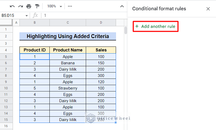
- Choose the data range to highlight duplicates. We chose Cell B5:D15. Select Add another rule from the Conditional format rules dialog box.
- After completing the previously mentioned steps, type the below formula into the Formula bar option, then click Done.
=(COUNTIF($D$5:$D$15,$D5)>3)*(COUNTIF($B$5:$D$15,$D5)>0)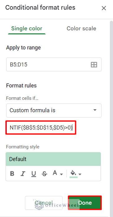
Formula Breakdown:
- COUNTIF($D$5:$D$15,$D5)>3
It will count the number of times each cell repeats in Column D and if any cell appears more than 3 times, it will highlight those.
- (COUNTIF($D$5:$D$15,$D5)>3)*(COUNTIF($B$5:$D$15,$D5)>0)
The second condition is added by the star (*) operator. COUNTIF($B$5:$D$15,$D5)>0 will highlight the entire row in the dataset.
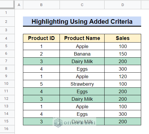
- All of the duplicates that appear more than 3 times in the Sales column are now highlighted.
Read More: Count Duplicates In Google Sheets (3 Ways)
Conclusion
We may want to highlight duplicate entries in different ways every time. In this article, we have shown you all possible ways of using formulas to highlight duplicates. You can follow any method based on your criteria and highlight duplicates. Besides, Google Sheets has a feature called added criteria by which you can highlight duplicates based on your specified criteria. Please feel free to leave any questions or suggestions in the comments section below. Visit our site Officewheel.com to explore more.
Related Articles
- How to Link Cells Between Tabs in Google Sheets (2 Examples)
- Use IF and OR Formula in Google Sheets (2 Examples)
- Google Sheets Use Filter to Remove Duplicates in Column
- How to Use ARRAYFORMULA in Google Sheets (6 Examples)
- VLOOKUP Multiple Columns in Google Sheets (3 Ways)
- How to Use SUM Function in Google Sheets (6 Practical Examples)
- Google Sheets: Convert Text to Number (6 Easy Ways)
- How to Apply a Custom Sort in Google Sheets