VLOOKUP can be used with the ARRAYFORMULA to do things that would save you plenty of time. ARRAYFORMULA, when used with the VLOOKUP function can fetch and show multiple data using just a single formula. In this article, we will try to show you how you can use ARRAYFORMULA with VLOOKUP in Google Sheets.
A Sample of Practice Spreadsheet
Download this practice spreadsheet to practice yourself
Why Use ARRAYFORMULA with VLOOKUP?
VLOOKUP looks for a particular value down the first column in a range of cells. It cannot return data from multiple columns. In such cases, ARRAYFORMULA can be used with VLOOKUP to return single or multiple columns of data.
ARRAYFORMULA can be used with non-array functions such as VLOOKUP which does not return data as an array and only returns a single result. So it can be incredibly useful when you want to show multiple columns as your result.
In the following examples, we will show you how you can use ARRAYFORMULA and VLOOKUP functions to return data as columns.
3 Scenarios to Use ARRAYFORMULA with VLOOKUP in Google Sheets
1. Return Single Column
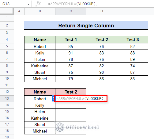
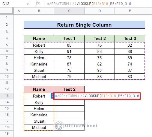
ARRAYFORMULA can be used with the VLOOKUP function to return a single column as result. For this, we have a dataset with student Names, and the marks achieved by the students in 3 different tests.
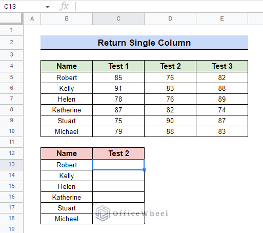
We will return the marks obtained by the students in Test 2 using these two functions. For this to look better, we have written the names of the students in a separate column. You can keep the names in their original place.
Steps:
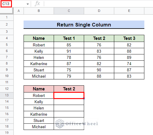
- First, go to the cell where you want to return the data. We go to cell C13 in our example.
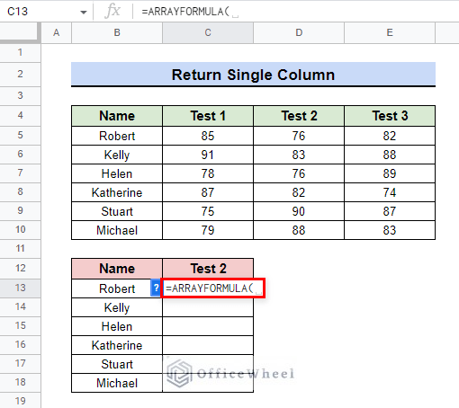
- Then, type in =ARRAYFORMULA( to return the data as a range.
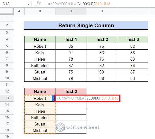
- Next, insert the VLOOKUP function to search for a value down the first column in the range of cells.
- After that, type in the range that you want to match to return the data. We type B13:B18 as this is the range of Names that we want to match for.
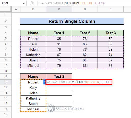
- Now, type in the range of your data table from where you want to look for the data. We type B5:E10 for our example.
- Next, type the column number of the table which you want to return. In our example, we type 3 as the data is in the third column of the table.
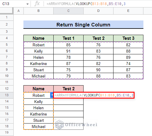
- Then, type 0 or FALSE to return the data if there is an exact match.
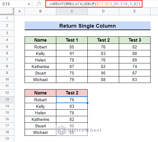
- The final formula is:
=ARRAYFORMULA(VLOOKUP(B13:B18,B5:E10,3,0))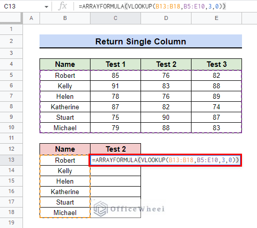
- Finally, press ENTER, and your data column is imported.
Read More: How to Fill Down an Entire Column in Google Sheets (4 Easy Ways)
Similar Readings
- How to Format Date with Formula in Google Sheets (3 Easy Ways)
- Use the DATEVALUE Function in Google Sheets (An Easy Guide)
- How to Compare Text in Google Sheets (3 Easy Ways)
- Use RIGHT Function in Google Sheets (6 Suitable Examples)
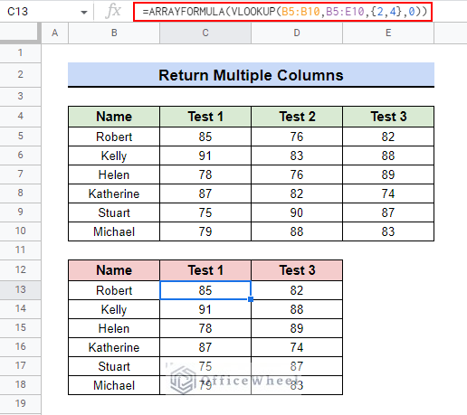
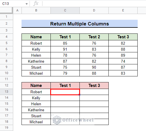
2. Return Multiple Columns
ARRAYFORMULA can be used with the VLOOKUP function to return two or more than two columns as result.
For this, we have a dataset with student Names, and the marks achieved by the students in 3 different tests. We will return the marks obtained by the students in Test 1 and Test 3 using these two functions.
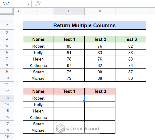
For this to look better, we have written the names of the students in a separate column. You can keep the names in their original place.
Steps:
- First, go to the cell where you want to show the result or return the columns. In our example, we go to cell C13.
- Then, type in the following formula:
=ARRAYFORMULA(VLOOKUP(B13:B18,B5:E10,{2,4},0))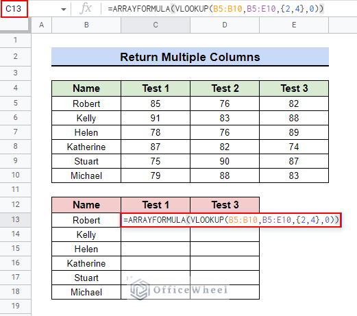
Formula Explanation:
- B13:B18 is the range we want to match to return the data.
- B5:E10 is the range of our data table from where we want to look for the data.
- {2,4} are the column numbers of the table which we want to return. Note that if there are more than one column, the column numbers must always be within the curly brackets to represent an array as a single value.
- 0 returns the data if there is an exact match.
- Finally, press ENTER to import your data columns.

Read More: How to Highlight Duplicates for Multiple Columns in Google Sheets
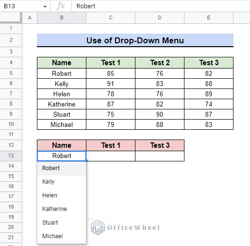
3. Using a Data Validation Drop-Down List
You can use ARRAYFORMULA with VLOOKUP by utilizing a drop-down menu.
Step 1: Creating a Drop-Down List with Data Validation
We have to create a drop-down list to validate data with ARRAYFORMULA and VLOOKUP. Follow these steps:
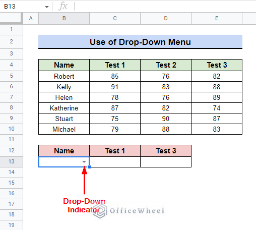
- First, select the cell where you want the drop-down list to appear. We select cell B13.
- Then, go to Menu Bar > Data > Data validation.
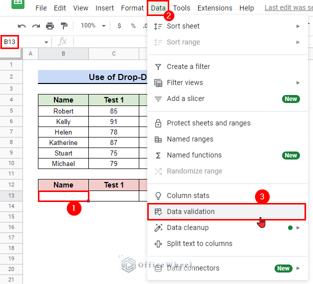
- Now, you will see the Data validation window appear.
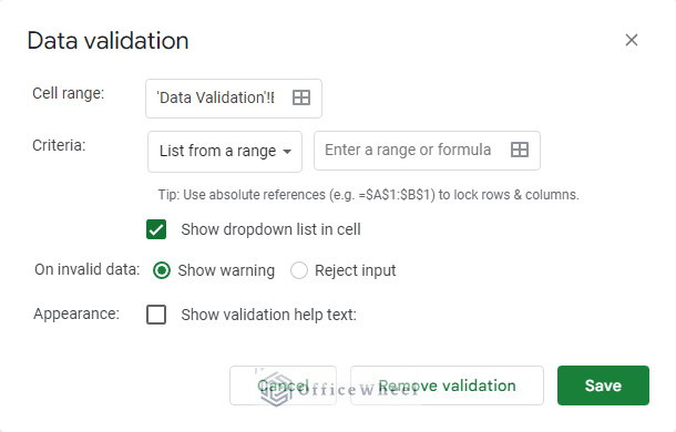
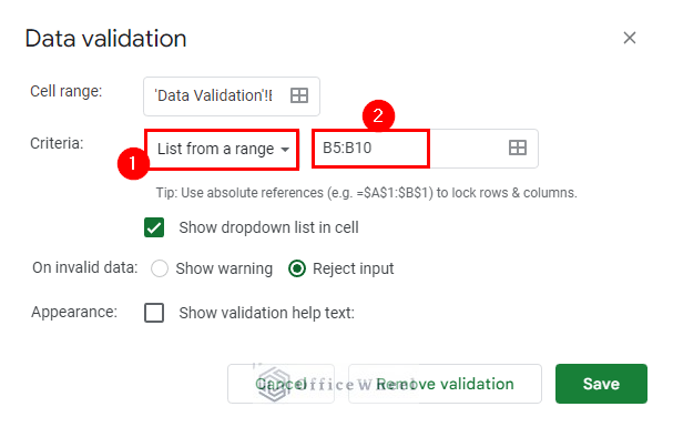
- Select List from a range from the Criteria drop-down options.
- Enter the range you want to make the drop-down list of. For our example, we type B5:B10.
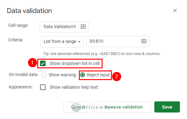
- Now, tick the Show dropdown list in cell option.
- After that, select Reject input for On invalid data.
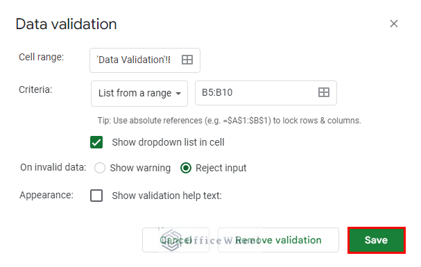
- Finally, press Save to have your drop-down list.
- The drop-down list will look like this at first:
Read More: How to Create Dependent Drop Down List in Google Sheets
Step 2: Applying VLOOKUP Formula for Drop-Down List
Now we have to create a custom formula for data validation.
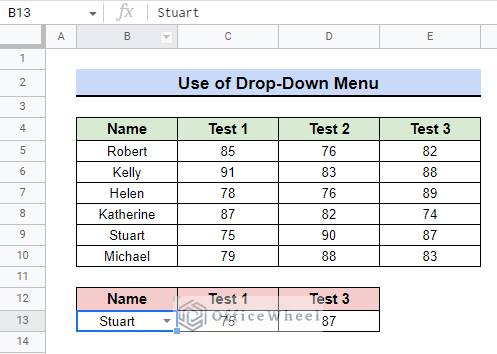
- First, select any name from the drop-down list. We selected the name Helen.
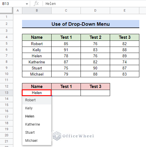
- After that, go to the cell where you want the validation to take place. We go to cell C13 in our example.
- Then type in the following formula:
=ARRAYFORMULA(IFERROR(VLOOKUP($B$13,B5:E10,{2,4},0)))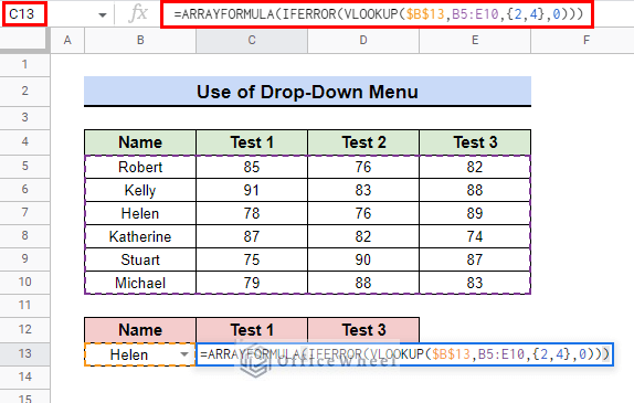
Formula Explanation:
- The formula we used to validate data is almost the same as before. The only exception is that, in this example, we used IFERROR along with ARRAYFORMULA and VLOOKUP. What IFERROR does is, it shows the exceptions if there are any. VLOOKUP shows empty cells as errors. Whereas, IFERROR shows them as empty cells.
- The cell B13 is used as the cell reference for the lookup condition that we want to match in the data table. We used the $ sign to lock the cell for absolute cell reference so that it does not change.
- Finally, press ENTER to have the marks obtained by Helen in Test 1 and Test 3. Navigate through the drop-down list names to show the necessary data.
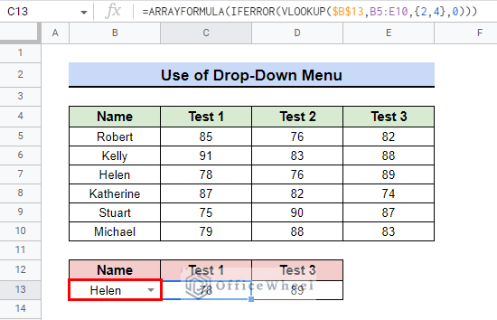
- If we select another name from the drop-down list say, for example, Stuart, then the marks obtained by Stuart will show.
Read More: Multi Row Dynamic Dependent Drop Down List in Google Sheets
Conclusion
In this article, we showed you how to use ARRAYFORMULA with VLOOKUP in Google Sheets. Keep practicing the examples that we have shown here for a better understanding of the concept. We hope this article was useful to you to help you.
Also, check out other articles on OfficeWheel to keep on improving your Google Sheets work knowledge.
Related Articles
- How to Link Cells Between Tabs in Google Sheets (2 Examples)
- Google Sheets Use Filter to Remove Duplicates in Column
- How to Use IF and OR Formula in Google Sheets (2 Examples)
- Google Sheets: How to Autofill Based on Another Field (4 Easy Ways)
- How to VLOOKUP Last Match in Google Sheets (5 Simple Ways)
- 2 Helpful Examples to VLOOKUP by Date in Google Sheets
- How to Ignore 0 for Standard Deviation Formula in Google Sheets