The VLOOKUP function is a popular and effective function in Google Sheets. Users apply this function quite often to find data from columns in large datasets. However, different errors happen while using this function. Among them, the N/A error is a common error. This error means that the look-up or search key is not available in the dataset. We can use the IF function with the VLOOKUP function to replace this error with a blank. In this article, we will discuss what to do if VLOOKUP shows a Not Found error in Google Sheets.
A Sample of Practice Spreadsheet
You can download the practice spreadsheet from the download button below.
3 Suitable Ways to Solve If VLOOKUP Not Found in Google Sheets
Suppose, you have a dataset that contains the names of some person names and their professions.
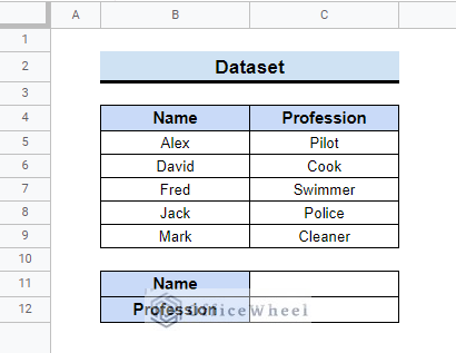
Now, you can easily find their profession using the VLOOKUP function. But sometimes if the data is not found in the dataset then you can use use the IF function to avoid showing errors. It replaces the error with a blank space or any text you want to put in the cell. Follow the article to learn what to do if VLOOKUP is not found in Google Sheets.
1. Using IFNA Function
You can use the IFNA function with the VLOOKUP function in Google Sheets to avoid showing the N/A error. The IFNA function returns the main value if there is no #N/A error, otherwise, it shows the second argument. Follow the steps below to learn how to do that by yourself.
📌Steps:
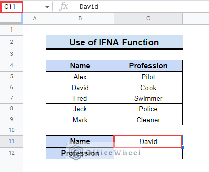
- First, insert a name from the dataset in cell C11.
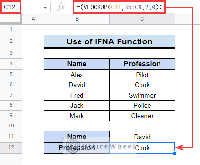
- Then, insert the following formula in cell C12.
=(VLOOKUP(C11,B5:C9,2,0))- Next, you will see the profession of the person in that cell.
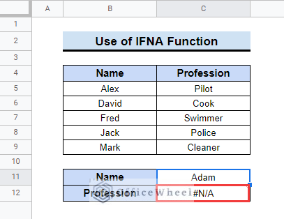
- After that, insert another name in cell C11, that is not in the dataset. Suppose, the name is Adam.
- Now, you will see the C12 cell is showing #N/A Because the name is not available in the dataset.
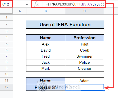
- Following, insert the below-mentioned formula in cell C12.
=IFNA(VLOOKUP(C11,B5:C9,2,0))- At this time, you will see that there is no error text in the cell. It is replaced with a blank.
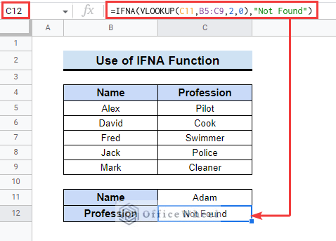
- Subsequently, you can also insert the following formula.
=IFNA(VLOOKUP(C11,B5:C9,2,0),"Not Found")- Then, the error will be replaced with the text “Not Found”.
Formula Breakdown:
- IFNA(VLOOKUP(C11,B5:C9,2,0)): If the formula returns #N/A error, then it will replace that with a blank space.
- IFNA(VLOOKUP(C11,B5:C9,2,0),”Not Found”): Here, the formula will show the VLOOKUP value if no #N/A error happens, otherwise it will show “Not Found”.
Read More: Alternative to Use VLOOKUP Function in Google Sheets
Similar Readings
- Combine VLOOKUP and HLOOKUP Functions in Google Sheets
- How to VLOOKUP All Matches in Google Sheets (2 Approaches)
- Create Hyperlink to VLOOKUP Cell in Multiple Rows in Google Sheets
- How to Use VLOOKUP Function for Exact Match in Google Sheets
- How to Use VLOOKUP to Import from Another Workbook in Google Sheets
2. Applying IFERROR Function
Another way to do this is to use the IFERROR with VLOOKUP function in Google Sheets. The IFERROR function returns the main value if there is no #N/A error, otherwise, it shows the second argument. Follow the steps below to know how to do that.
📌Steps:
- First, select cell C12 and insert the VLOOKUP formula.
=(VLOOKUP(C11,B5:C9,2,0))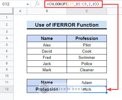
- Then, insert the below IFERROR formula.
=IFERROR(VLOOKUP(C11,B5:C9,2,0))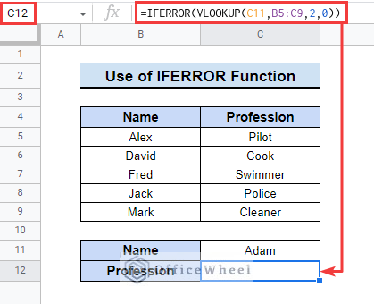
But, it is better to avoid IFERROR in this case, as it will return 0/blank for any kind of error in the dataset other than the not found error.
Read More: How to Use IFERROR with VLOOKUP Function in Google Sheets
3. Utilizing ISNA Function
You can also use the ISNA function with the IF function to replace the error message. The ISNA function checks if there is a #N/A error. Follow the below-mentioned steps to do that by yourself.
📌Steps:
- First, insert the VLOOKUP formula in cell C12. You will see the #N/A error in the cell.
=(VLOOKUP(C11,B5:C9,2,0))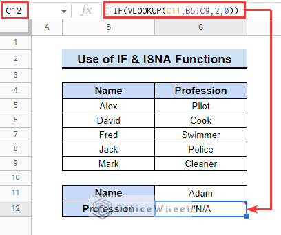
- Now, insert the following formula with the ISNA function.
=IF(ISNA(VLOOKUP(C11,B5:C9,2,0))=TRUE,0,VLOOKUP(C11,B5:C9,2,0))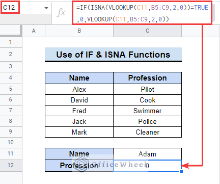
- Next, you can also replace the 0 with text or blank. Just insert the formula below.
=IF(ISNA(VLOOKUP(C11,B5:C9,2,0))=TRUE,"Not Found",VLOOKUP(C11,B5:C9,2,0))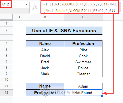
- ISNA(VLOOKUP(C11,B5:C9,2,0): This formula will return the #N/A error in the cell if there is no lookup value available.
- IF(ISNA(VLOOKUP(C11,B5:C9,2,0))=TRUE,0,VLOOKUP(C11,B5:C9,2,0)): If the formula shows #N/A error then the formula is TRUE, so it will return 0. However, if no #N/A error happens it will return the VLOOKUP
- IF(ISNA(VLOOKUP(C11,B5:C9,2,0))=TRUE,”Not Found”,VLOOKUP(C11,B5:C9,2,0)): Same as the above formula, this time it will return the text “Not Found” instead of 0.
Read More: VLOOKUP Error in Google Sheets (with Quick Solutions)
Things to Remember
- Please keep in mind, the VLOOKUP function searches the value from the first column of the data table.
Conclusion
We have tried to show you what to do if VLOOKUP is not found in Google Sheets. Hopefully, the examples above will be enough for you to understand how to resolve this issue. Please use the comment section below for further queries or suggestions. You may also visit our OfficeWheel blog to explore more about Google Sheets.
Related Articles
- Google Sheets Vlookup Dynamic Range
- How to Use VLOOKUP with Named Range in Google Sheets
- How to Use Wildcard in Google Sheets (3 Practical Examples)
- How to Use Nested VLOOKUP in Google Sheets
- How to Check If Value Exists in Range in Google Sheets (4 Ways)
- How to VLOOKUP for Partial Match in Google Sheets
- How to Use VLOOKUP for Conditional Formatting in Google Sheets
- How to Use VLOOKUP with Drop Down List in Google Sheets