Date formats in Google Sheets usually depend on the regional or locale settings. Most commonly mm/dd/yyyy for the United States and dd/mm/yyyy for the United Kingdom locale.
While there are other formats of dates that the application recognizes, these are the two fundamental ones. This means that if you want to change a date format for the long run then change the locale settings.
A shortcut to this is to use formulas to format a date in Google Sheets, as the functions can take the underlying date value and transform it to the user’s requirements.
Let’s see how it’s done.
3 Ways to Format Date with Formula in Google Sheets
1. Use the DATE Function to Insert a Date Regardless of Format in Google Sheets
First up we have is DATE. It is a simple function that takes three arguments: Year, Month, and Day.
DATE(year, month, day)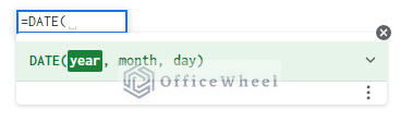
Like most functions in Google Sheets, DATE is dependent on its arguments to work. The advantage of this is that the function is taking the year, month, and day values of a date and outputting it in the default date format of the spreadsheet.
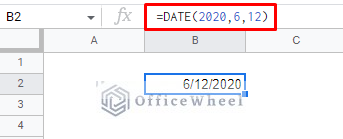
Since the output always shows in the default format, dates applied this way are not affected by regional settings as the spreadsheet is moved from one user to another in different regions.
This opens up a lot of ways we can insert a date in Google Sheets, regardless of their original formatting.
Here’s an example with cell reference:
We have different date values in different cells in a dataset. We will form a date in the default format using the DATE function.
=DATE(D3,C3,B3)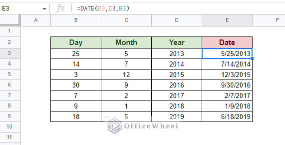
Example: Extract from an Existing Date that is in the Wrong Format
In the following dataset, we have a list of dates in the dd/mm/yyyy format. Since our locale is the United States, this format is considered wrong and is seen as a text value.
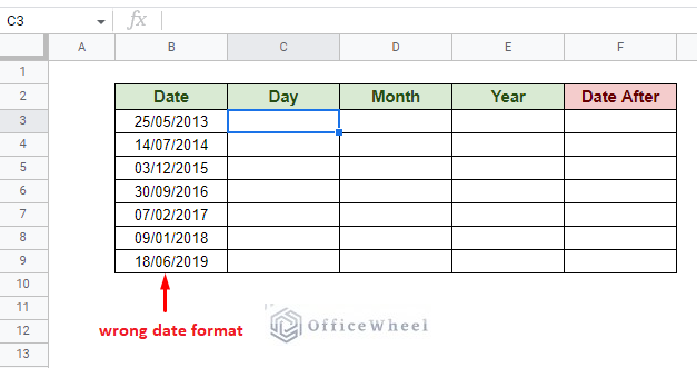
We will use the DATE formula to convert it to the correct format, mm/dd/yyyy.
Step 1: Split the date into their respective day, month, and year values.
To get the Day value, we use the LEFT function:
=LEFT(B3,2)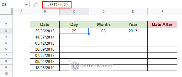
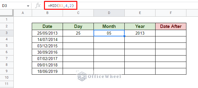
For month, we use the MID function:
And finally, for the year value, we use the RIGHT function:
=RIGHT(B3,4)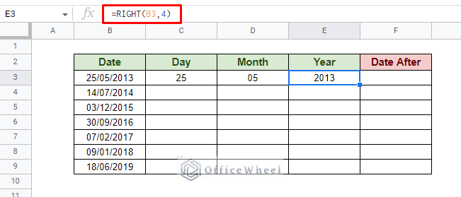
Apply the formulas to the rest of their respective columns with the fill handle.
Step 2: Use the DATE function to bring them all together.
=DATE(E3,D3,C3)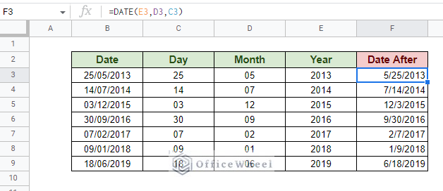
The great thing about functions is that we can combine them together to create an equally sensible formula.
This the combined formula, omitting the need for the Day, Month, and Year columns will look like this:
=DATE(RIGHT(B3,4),MID(B3,4,2),LEFT(B3,2))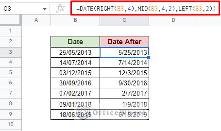
Read More: Convert Date to Month and Year in Google Sheets (A Comprehensive Guide)
2. Use DATEVALUE Formula to Format Date in Google Sheets
We continue our article with the next approach which uses the DATEVALUE function as its core.
DATEVALUE(date_string)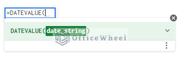
There are many valid formats of dates in Google Sheets. Some of them are numbers, text, or even a combination of both.
The DATEVALUE function essentially returns the underlying value of the date as long as the date has one of these valid date formats.
=DATEVALUE(B3)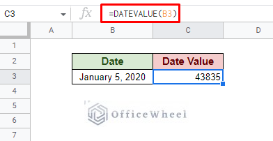
Now, we can take this base value and format it in any way we want.
For example, we can combine the TO_DATE function with DATEVALUE to create a formula that formats the date into the default date format in Google Sheets:
=TO_DATE(DATEVALUE(B3))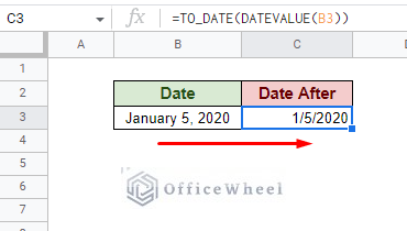
Example: Converting a String to a Date in Google Sheets
We have the following dataset:
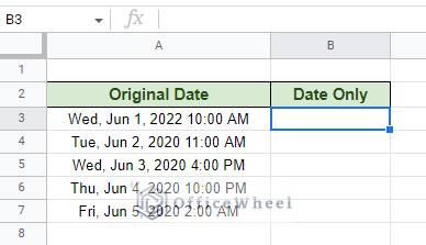
What we want to do is extract only the date portion of the strings and present them in the default date format. Let’s see how it’s done.
Step 1: Use the MID function to determine the location of the date in the string.
MID(A3,6,11)Combine it with the DATEVALUE function to output the underlying date value of the extracted date.
=DATEVALUE(MID(A3,6,11))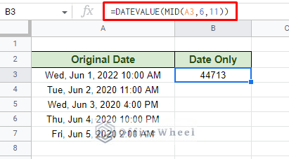
Step 2: Update the column with the default date format from the toolbar. You can apply custom formats as well. Let’s take it a step further and apply the formatting to the whole column to accommodate for the other dates.
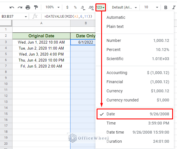
Step 3: At this point, we can simply use the fill handle to extract all the adjacent strings to the proper date format.
But instead of just one cell, we will take the cell range of the Original Date column into account, A3 to A3:A. And to accommodate this cell range, we must put the formula inside ARRAYFORMULA.
=ArrayFormula(IFERROR(DATEVALUE(MID(A3:A,6,11)),))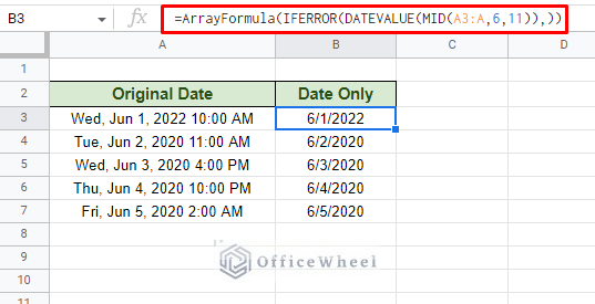
Note: We’ve used the IFERROR function to accommodate any blank cells in column A.
Read More: How to Format Date with Formula in Google Sheets (3 Easy Ways)
3. Use TEXT Formula to Format Date in Google Sheets
If having the date as a text or a string is not an issue, this method is the best way to convert any date to the desired date format in Google Sheets. That is by using the TEXT function.
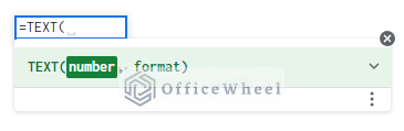
This function can take any number in Google Sheets, including any valid date, and convert them to the desired format.
For date formatting, the format argument of the TEXT function is where the magic happens. With the correct format code for the day, month, or year, we can format any date using the TEXT formula in Google Sheets.
Here is a list of format codes and their outputs:
| Date Format Code | Result |
|---|---|
| dd-mm-yyyy | 25-2-2022 |
| mm/dd/yyyy | 2/25/2022 |
| MMMM d, YYYY | February 2, 2022 |
| dd-MMM-YYYY | 02-Feb-2022 |
| MMM d, YYYY | Feb 2, 2022 |
| mmm-yy | Feb-22 |
| dd MMM YYYY | 02 Feb 2022 |
| dddd | Wednesday |
| ddd, MMMM DD YYYYY | Wed, February 02 2022 |
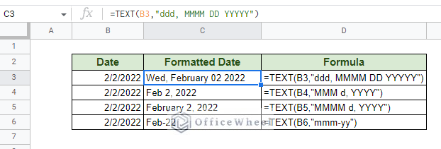
A few examples in the spreadsheet:
Read More: How to Convert Text to Date in Google Sheets (3 Easy Ways)
Final Words
Depending on user requirements, any of the three approaches discussed above can be used to format a date with their respective formulas in Google Sheets quite effectively. Of which the TEXT function stands out with the most customizability, only if having the result as a string is of no issue.
Feel free to leave any queries or advice you might have in the comments section below.
Related Articles
- Find Number of Days in a Month in Google Sheets (An Easy Guide)
- Convert Date to Month and Year in Google Sheets (A Comprehensive Guide)
- Add 7 Days to Date in Google Sheets (And More)
- Calculate Days Between Dates in Google Sheets (5 Easy Ways)
- How to Organize Google Sheets by Date (3 Easy Ways)
- Find if Date is Between Dates in Google Sheets (An Easy Guide)
- How to Add Months to a Date in Google Sheets (2 Easy Ways)