How to VLOOKUP Multiple Columns in Google Sheets (3 Ways)

VLOOKUP is a vertical lookup that we use when we need to find a value row-wise within columns in a table. For example, we can use VLOOKUP to find a Brand Name from a dataset with the brand’s corresponding products, product ID, price, etc. The VLOOKUP function allows us to find the required data from single and multiple columns. This article will teach us how to VLOOKUP multiple columns in Google Sheets.

A Sample of Practice Spreadsheet

Introduction to VLOOKUP Function in Google Sheets

The VLOOKUP function looks at a particular value to return corresponding values. For example, if you VLOOKUP a brand name in a dataset, you can find the corresponding product name, ID, price, etc.

Syntax:

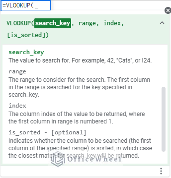
Inputs:

• search_key: This is the value to look up for. For example, if we consider cell B2 as search_key then VLOOKUP will start from cell B2.
• range: This criterion indicates the range to look up in. If we want to pull data from column C then the range will be column C.
• index: This parameter represents the column number from the range according to search_key. For example, if the range is columns C:F and you need data from column E, then index will be 3. As C=1, D=2, and E=3.
• [is_sorted]: You must sort the range to the exact match. Here, FALSE or 0 means Exact Match, and TRUE or 1 means Approximate Match.

Return Value:

• Returns the first matching value from the lookup range.

Read More: Google Sheets Vlookup Dynamic Range

3 Suitable Ways to VLOOKUP Multiple Columns in Google Sheets

Here we will show 3 different ways to VLOOKUP multiple columns in Google Sheets using different datasets. So let’s start!

1. Applying Combined Search Criteria

The dataset below contains Brand and Product, Product ID, and Price. Here, we will apply combined search criteria to search for Gucci Hand Bag and get the corresponding price.

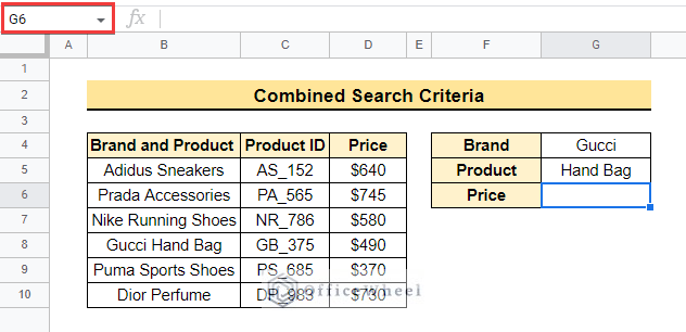
• First select cell G6 to insert the following formula into the cell. Then you will get the desired result as follows.

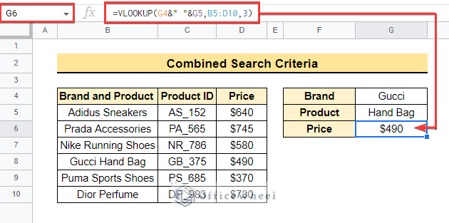
• Here G4&” “&G5 in the formula concatenates cell G4 and G5 separated by a space and returns Gucci Hand Bag. The VLOOKUP function uses this output as the search_key.

Read More: Combine VLOOKUP and HLOOKUP Functions in Google Sheets

2. Using Helper Column

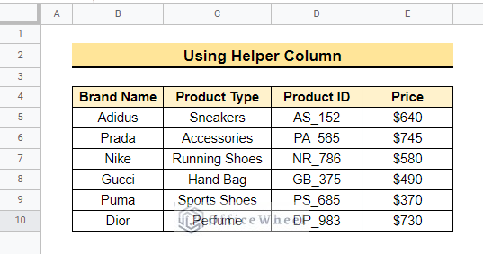
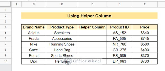
The dataset below contains Brand Name, Product Type, Product ID, and Price. Here, we will VLOOKUP multiple columns using a helper column. The steps are mentioned below.

📌 Steps:

• First, insert a new column before the Product ID column in the actual dataset as below.

• Then, insert the following formula into cell D5 to get the output as follows.

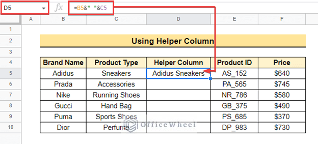
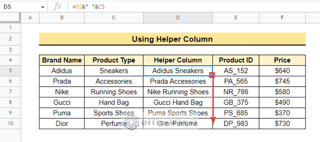
• Next drag down the fill handle icon to copy the formula below.

• You can hide the helper column if you want. After that, select cell C13 to insert a VLOOKUP formula lookup for the value in cell B13.

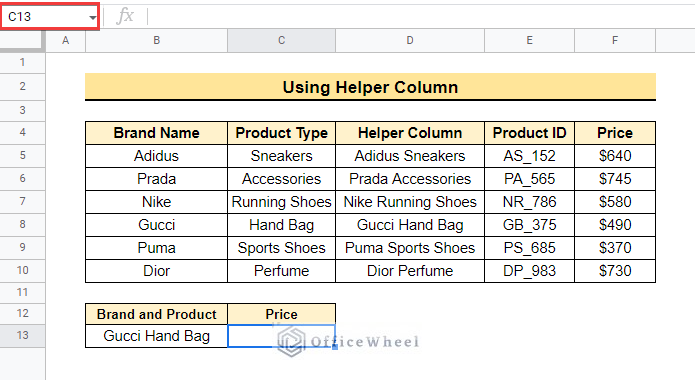
• Now, enter the following formula in that cell to get the output below.

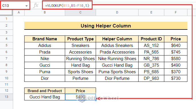
Read More: Highlight Duplicates for Multiple Columns in Google Sheets

Similar readings

• How to Use IFERROR with VLOOKUP Function in Google Sheets
• Use VLOOKUP with Named Range in Google Sheets
• How to Use Nested VLOOKUP in Google Sheets
• Use ARRAYFORMULA with IF Function in Google Sheets

3. Utilizing ARRAYFORMULA

The ArrayFormula function in Google Sheets enables non-array formulas to return values in multiple rows and columns. Here we will use this function with the VLOOKUP function to avoid inserting a helper column as in the earlier method to get the desired output.

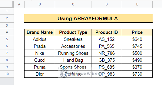
• First, select cell D13 and apply the formula given below.

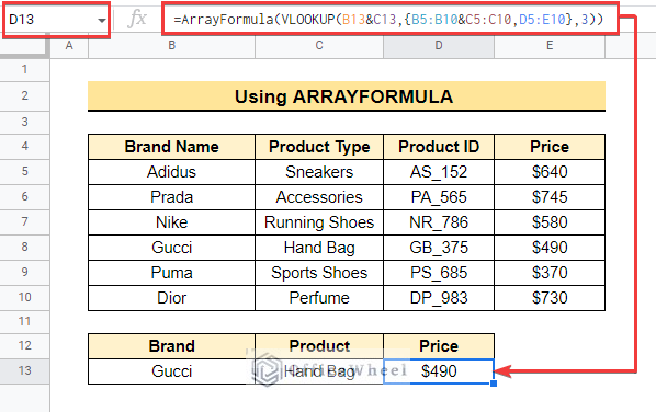
• Here B13&C13 in the formula concatenates the cells to return Gucci Hand Bag as the Then the array {B5:B10&C5:C10,D5:E10} returns an array of 3 columns containing Brand and Product, Product ID, and Price.

Read More: How to Use ARRAYFORMULA with VLOOKUP in Google Sheets

How to VLOOKUP to Return Multiple Columns in Google Sheets

Here will show how you can use the VLOOKUP function to return multiple columns at once in Google Sheets.

Suppose you want to insert the VLOOKUP formula in cell C13 to return the Product ID and Price at the same time for the corresponding search_key in cell B13.

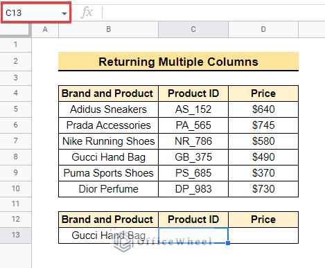
• First, select cell C13 and enter the following formula to get the output below.

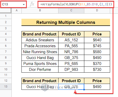
• Here the array {2,3} replaces the single index argument in the earlier methods to return multiple columns at the same time.

Read More: How to VLOOKUP with Multiple Criteria in Google Sheets

Things to Remember

• Always remember to select the correct data range as VLOOKUP does not allow you to have any blank data while selecting the range.
• You can press CTRL + SHIFT + ENTER to convert a non-array formula to an ArrayFormula in Google Sheets.

Conclusion

In this article, we explained the anatomy of the VLOOKUP function. We also explained how to VLOOKUP multiple columns in Google Sheets in different ways. Hopefully, the methods will help you to apply the function to your own dataset. Please let us know in the comment section if you have any further queries or suggestions. You may also visit our OfficeWheel blog to explore more Google Sheets-related articles.

Related Articles

• How to Use IF and OR Formula in Google Sheets (2 Examples)
• Google Sheets: How to Autofill Based on Another Field (4 Easy Ways)
• How to VLOOKUP Last Match in Google Sheets (5 Simple Ways)
• 2 Helpful Examples to VLOOKUP by Date in Google Sheets
• How to Ignore 0 for Standard Deviation Formula in Google Sheets
• Multi Row Dynamic Dependent Drop Down List in Google Sheets
• How to Create Dependent Drop Down List in Google Sheets
• Alternative to Use VLOOKUP Function in Google Sheets