We are familiar with using VLOOKUP with single criteria but sometimes we need to do it with multiple criteria. There are many ways to VLOOKUP with multiple criteria in google sheets. But we’ll use the VLOOKUP function and other functions to show 4 easy methods to VLOOKUP with multiple criteria in Google Sheets by clear images and steps.
4 Simple Methods to VLOOKUP with Multiple Criteria in Google Sheets
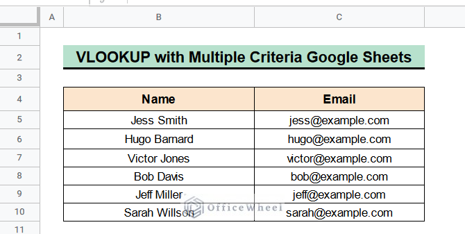
First, let’s get introduced to our dataset. Here we can see the names and emails of some people. Now we will see how the VLOOKUP function works in multiple criteria.
1. Single Column VLOOKUP with Multiple Criteria in Google Sheets
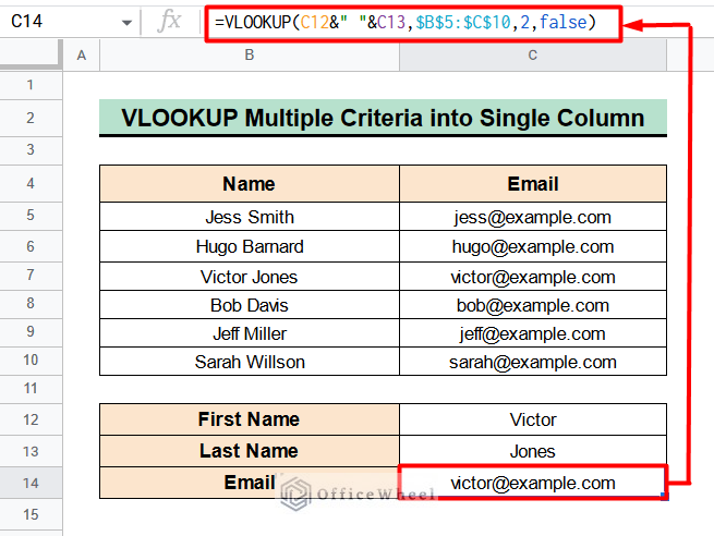
In the first method, we will use the VLOOKUP function to match multiple criteria into a single column. This method is useful when we have a single-column dataset but want to get results for two combined data sets. In this case, we have the first name and last name. We will find the corresponding email address from our data set.
Steps:
- Type the following formula in Cell C14–
=VLOOKUP(C12&" "&C13,$B$5:$C$10,2,false)- Hit Enter button to get the result automatically. If you write any first name in Cell C12 and the last name in Cell C13, you will get their email quickly.
Read More: How to VLOOKUP Multiple Columns in Google Sheets (3 Ways)
2. VLOOKUP for Multiple Criteria Using Helper Column
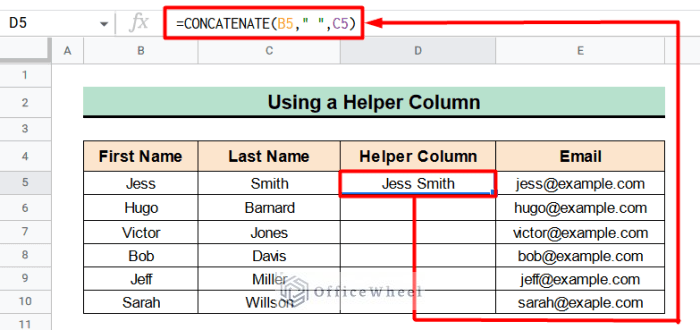
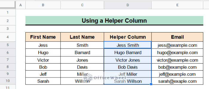
Moreover, we can also use a helper column to VLOOKUP multiple criteria if we have a different data set. This method is contrary to the previous process. Because using this method we can get results for a single column of data if we have data in two different columns. Like in this dataset we have the first names and last names separately. So we have to create a helper column by using the CONCATENATE function.
Steps:
- Apply the following formula in Cell D5-
=CONCATENATE(B5," ",C5)- Press Enter button and you will get the names together.
- Then assign the Fill Handle tool to fit the formula in the whole column.
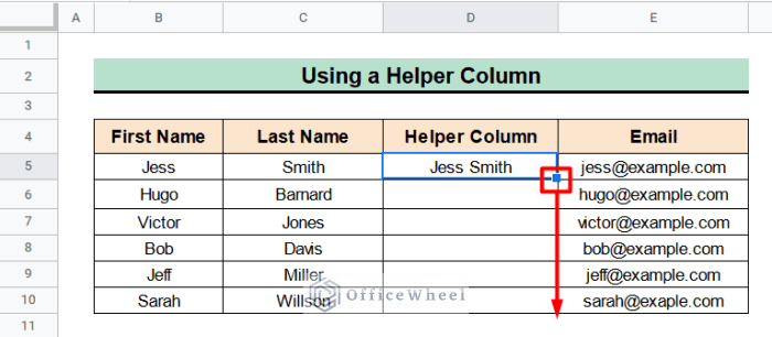
- You will get the names together in the whole column.
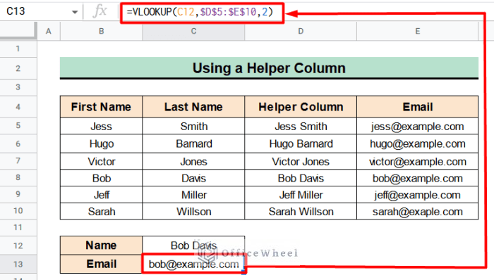
- Now we’ll apply the VLOOKUP function to extract the final output, so write the following formula in Cell C13–
=VLOOKUP(C12,$D$5:$E$10,2)- Press Enter button and you will finally get the corresponding email address.
Read More: How to Use Formula to Highlight Duplicates in Google Sheets
Similar Readings
- How to Sum Using ARRAYFORMULA in Google Sheets
- Google Sheets: How to Autofill Based on Another Field (4 Easy Ways)
- How to Use ARRAYFORMULA in Google Sheets (6 Examples)
- Create Hyperlink to VLOOKUP Cell in Multiple Rows in Google Sheets
- How to Use Nested VLOOKUP in Google Sheets
3. Merge ARRAYFORMULA and VLOOKUP Functions for Multiple Criteria
Alternatively, we can use the ARRAYFORMULA function to find multiple criteria in google sheets. This method is much easier, unlike the previous method. We can get results with just one click.
Steps:
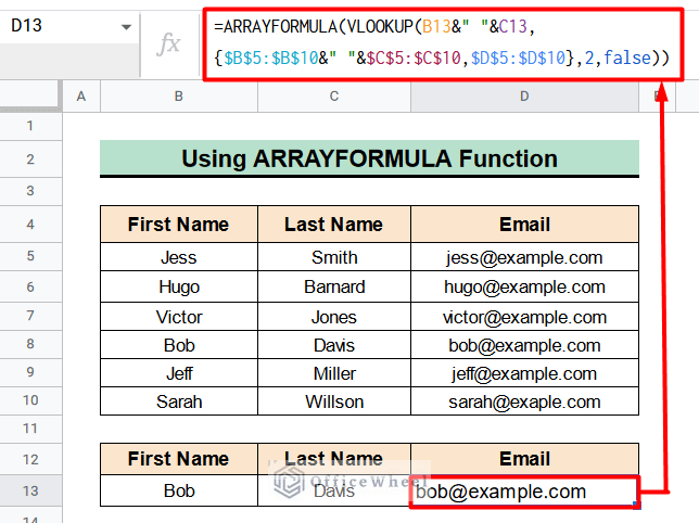
- Type the following formula in Cell D13–
=ARRAYFORMULA(VLOOKUP(B13&" "&C13, {$B$5:$B$10&" "&$C$5:$C$10, $D$5:$D$10},2,false))- Hit Enter button to get the result.
Formula Breakdown:
- VLOOKUP(B13&” “&C13,{$B$5:$B$10&” “&$C$5:$C$10,$D$5:$D$10},2,false)
Firstly, the VLOOKUP function will search for the first name in Column B and the last name in Column C together and give the value of the email in Column D.
- ARRAYFORMULA(VLOOKUP(B13&” “&C13,{$B$5:$B$10&” “&$C$5:$C$10, $D$5:$D$10},2,false))
Finally, the ARRAYFORMULA function will perform multiple calculations together and give the correct result.
Read More: How to Use ARRAYFORMULA with VLOOKUP in Google Sheets
4. Apply FILTER Function to VLOOKUP with Multiple Criteria in Google Sheets
We can also apply the FILTER function instead of VLOOKUP to get multiple criteria in google sheets very easily. This method is handy because the formula is straightforward.
Steps:
- Apply the following formula in Cell D13–
=FILTER($D5:$D10,B13=$B5:$B10,C13=$C5:$C10)- Hit Enter button to get the result. If you change the first and last name, you will get the corresponding email automatically.

Read More: Google Sheets Use Filter to Remove Duplicates in Column
Conclusion
That’s all for now. Thank you for reading this article. In the article, you will find 4 useful methods to VLOOKUP with multiple criteria in Google Sheets. If you have any queries please leave a comment in the comment section. You will also find different articles related to google sheets on our officewheel.com Visit the site and explore more.
Related Articles
- How to Use VLOOKUP with Named Range in Google Sheets
- Google Sheets Vlookup Dynamic Range
- How to Use IF and OR Formula in Google Sheets (2 Examples)
- [Fixed!] Google Sheets If VLOOKUP Not Found (3 Suitable Solutions)
- How to VLOOKUP for Partial Match in Google Sheets
- VLOOKUP Between Two Google Sheets (2 Ideal Examples)
- How to Use ARRAYFORMULA with IF Function in Google Sheets