Highlighting cell if value exists in another column is often helpful to identify common data of different columns. One can easily highlight cell in Google Sheets if value exists in another column using conditional formatting and custom functions. In this article, we discuss three different custom functions to do that.
A Sample of Practice Spreadsheet
You can download the practice sheet from the link below. After downloading you can practice on your own as we demonstrate here.
3 Ways to Highlight Cell If Value Exists in Another Column in Google Sheets
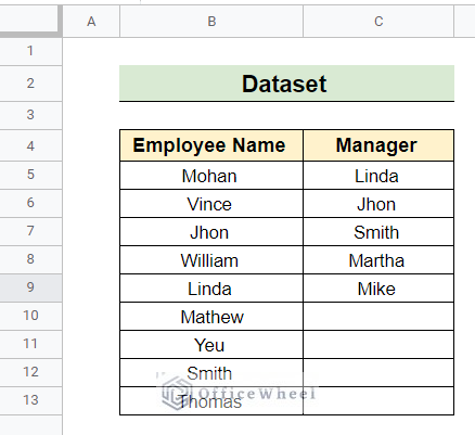
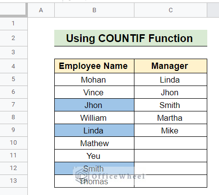
First, we have to look at our dataset. Our dataset contains two columns namely Employee Name, and Manager. Now, we want to highlight cells of the Employee Name column if the employee name exists in the Manager column.
1. Applying MATCH Function
There are multiple techniques in Google Sheets to highlight cell if value exists in another column. Here is a quick demonstration of using the MATCH function with conditional formatting to do that. Basically, MATCH function tells us the position of specific value within a range.
Steps:
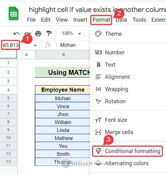
- First of all, select the cell or range of cells you want to highlight if they exist in another column.
- Then click Format from the menu bar and finally select Conditional formatting.
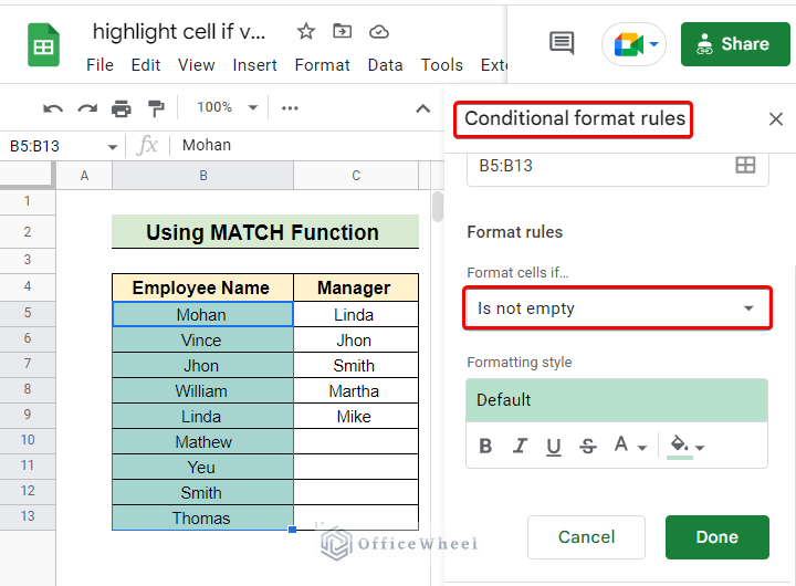
- After selecting conditional formatting you will get a small window at the upper right portion of the current window called Conditional format rules. Within Format rules of the small window, there is a box Format cells if… which is ‘Is not empty’ by default.
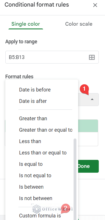
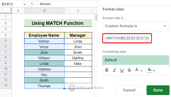
- Now, we click the format cells if.. box and set the Format rules as ‘Custom formula is’.
=MATCH(B5,$C$5:$C$7,0)>0- Just below the ‘Custom formula is’ a formula box appeared as indicated. Now, insert the above formula in the formula box.
Formula Breakdown
- B5 is the search key.
- $C$5:$C$7 indicates the static range of cells over which the MATCH function searches the search key.
- Here search type is 0 because we want an exact match.
- The MATCH function returns the position of the matched value which is always greater than 0 if matched. Hence, highlight the matched cells.
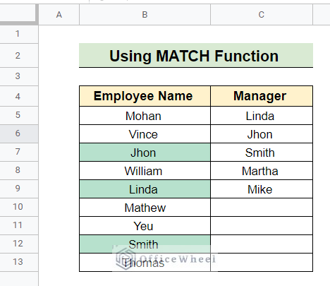
- Click on Done to highlight the desired cells. Finally, we got our desired cells highlighted below.
Read More: Google Sheets IF Statement in Conditional Formatting
2. Using VLOOKUP Function
The VLOOKUP Function can be used as the MATCH function for the same task. The VLOOKUP function is a build-in function in Google Sheets to search across columns. There are two ways of using the VLOOKUP function to highlight the cells if value exists in another column in Google Sheets.
2.1 Combining NOT, ISERROR and VLOOKUP Functions
Here, we will use ISERROR and NOT functions along with the VLOOKUP function. The ISERROR function returns TRUE or FALSE based on the value of its argument. On the other hand, the NOT function alters a boolean value.
Steps:
- Firstly, select the cell range you want to highlight. Here the range is B5:B13.
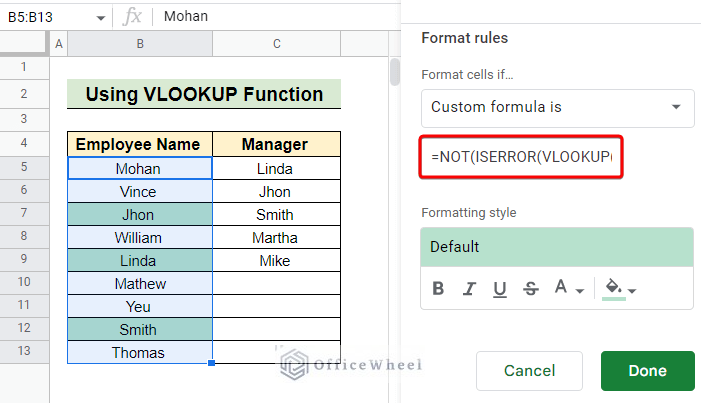
- Then select Format >>Conditional Formatting >> Custom formula is as earlier.
=NOT(ISERROR(VLOOKUP($B5,$C$5:$C$7,1,FALSE)))- Insert the above formula in the formula box that appeared below the ‘Custom formula is’.
Formula Breakdown
- $B5 is the search key.
- $C$5:$C$7 indicates the static range of cells over which the VLOOKUP function searches the search key.
- Here index 1 means it searches over the first column of the search range, the only column in our search range.
- Finally, FALSE means we want an exact search, not an approximate one.
- VLOOKUP function returns values passed by the ISERROR function which returns TRUE for all unmatched cells and FALSE for matched cells.
- At last, these boolean values pass as the argument of the NOT function. This returns FALSE for all the cells of the Employee Name column that are not in the Manager column, hence highlighted.
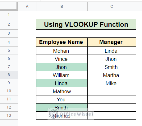
- After clicking on Done we got our desired cells highlighted as below.
Read More: How to Use the VLOOKUP Function in Google Sheets
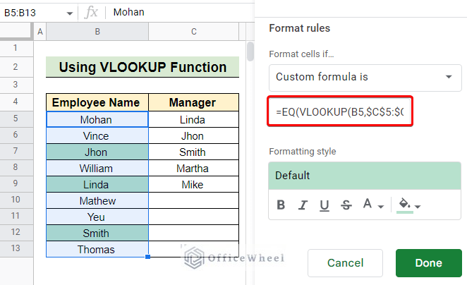
2.2 Utilizing VLOOKUP and EQ Functions
The VLOOKUP function and the EQ function together can perform similar tasks of highlighting cells. The EQ function compares its two arguments to whether they are equivalent or not.
Steps:
- Initially, select the cell range you want to highlight.
- Then select Format >>Conditional Formatting >> Custom function is as we have done already.
=EQ(VLOOKUP(B5,$C$5:$C$7,1,FALSE), B5)- Just below the ‘Custom formula is’ insert the above formula in the formula box.
Formula Breakdown
- B5 is the search key.
- $C$5:$C$7 indicates the static range of cells over which the VLOOKUP function searches the search key.
- Here index 1 means it searches over the first column of the search range, the only column in our search range.
- Finally, FALSE means we want an exact search, not an approximate one.
- The EQ function takes the return value of the VLOOKUP function and B5 as an argument and compares them.
- The EQ function returns TRUE and highlights the cell if it is equal to the VLOOKUP function’s return value.
- Click on Done to highlight the desired cells. Finally, we got our desired cells highlighted below.
Read More: How to Use VLOOKUP for Conditional Formatting in Google Sheets
Similar Readings
- How to Use VLOOKUP with IF Statement in Google Sheets
- Use Nested IF Function in Google Sheets (4 Helpful Ways)
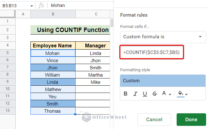
3. Implementing COUNTIF Function
The next and last way of highlighting the cells if value exists in another column is by implementing the COUNTIF function. The COUNTIF function counts cells within a range based on given criteria.
Steps:
- Firstly, select the cell range you want to highlight.
- Then select Format >>Conditional Formatting >> Custom formula is in a similar fashion.
=COUNTIF($C$5:$C7,$B5)- Just below the ‘Custom formula is’ a formula box appeared. We insert the above formula in the formula box as shown in the image.
Formula Breakdown
- $C$5:$C$7 is the criteria range.
- $B5 is the criteria.
- The COUNTIF function returns the number of occurrences of the criteria within the criteria range and highlights criteria if the occurrence does not equal 0.
- You can change the color of the highlighted cells by clicking on the red box within the formatting style as indicated.
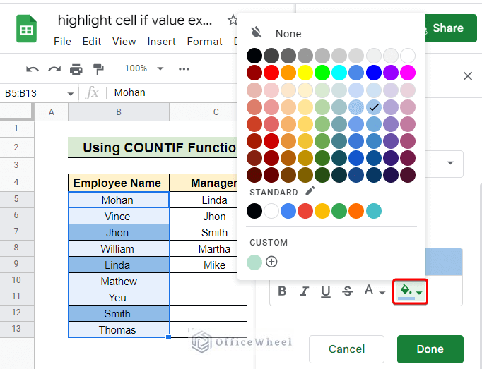
We select the light blue color for highlighting and then click on Done to highlight cells of column B that also exist in column C.
Read More: How to Use IF Function in Google Sheets (6 Suitable Examples)
Things to Remember
- Always remember to select the correct data range for each of the functions.
- Don’t be confused with the final boolean values of using the VLOOKUP function. Conditional formatting is different for different combinations of functions.
Conclusion
In conclusion, I hope that we have covered most of the customs functions of highlighting cell if value exists in another column in Google Sheets. Furthermore, If you have any questions regarding this article feel free to comment below and I will try to reach out to you soon. Visit our website OfficeWheel for many useful articles.
Related Articles
- How to Do IF THEN in Google Sheets (3 Ideal Examples)
- Use Nested IF Statements in Google Sheets (3 Examples)
- How to Use IF and OR Formula in Google Sheets (2 Examples)
- Cell Contains Text Then Return Value in Another Cell in Google Sheets
- How to Use Multiple IF Statements in Google Sheets (5 Examples)