Use INDEX MATCH Across Multiple Sheets in Google Sheets

INDEX MATCH makes it easier to find the data you need, especially if you have multiple sheets across Google Sheets from which to retrieve data. Google Sheets VLOOKUP is typically used when you need to locate data in your sheet that matches a specific key record. However, VLOOKUP has its limitations. You should therefore learn INDEX MATCH to boost your skills for the job.

A Sample of Practice Spreadsheet

You can copy the spreadsheet that we’ve used to prepare this article.

Step by Step Process to Use INDEX MATCH Across Multiple Sheets in Google Sheets

To show how to use the INDEX and MATCH functions jointly, we must first have a dataset. To walk you through the procedure step by step, we’ll utilize the dataset featured below.

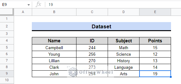
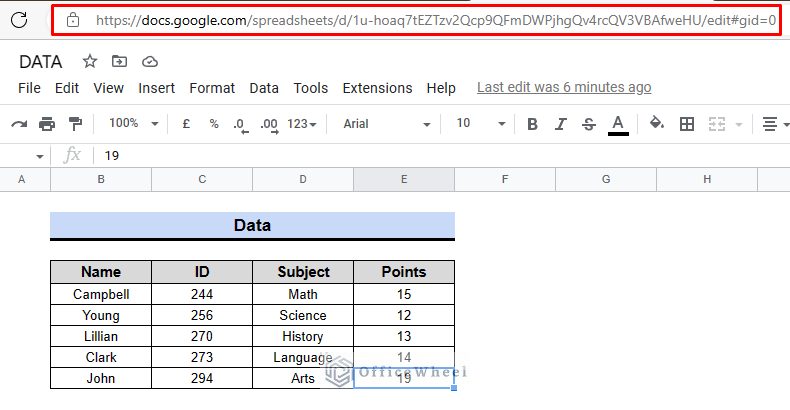
Assume we have a dataset of a few students that includes information about their ID number, the subjects they excel in, and the points they earned in those core subjects.

Step 1: Using the INDEX Function to Lookup Values

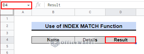
• We will first open three headers, for example, Name, Details, and Result. We will use cells B4, C4, and D4 in this case, correspondingly.

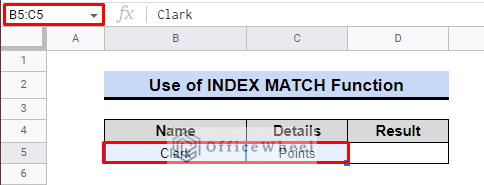
• To gather the information that we will search for later, we will use the cells B5, C5, and D5 below.
• Assume we are looking for how many points Clark receives in the subject in which he excels. So, underneath the Name header, we will write Clark, and below the Details header, we will write Points.

• Now, in cell D5, we will use the INDEX Function to retrieve the point he was awarded.

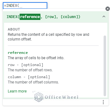
• We will first establish a data reference to aid in the search query. For this example, the reference data is in the Data sheet.
• Check the following formula,

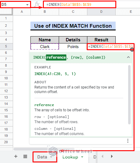
Read More: Find All Cells With Value in Google Sheets (An Easy Guide)

Step 2: Finding Row Number Using MATCH Function

• Now, using the MATCH function, we will choose the row value for the INDEX function.
• First, we’ll use the MATCH function to choose the cell that will be compared to the values in the row. It is cell B5 in this situation.

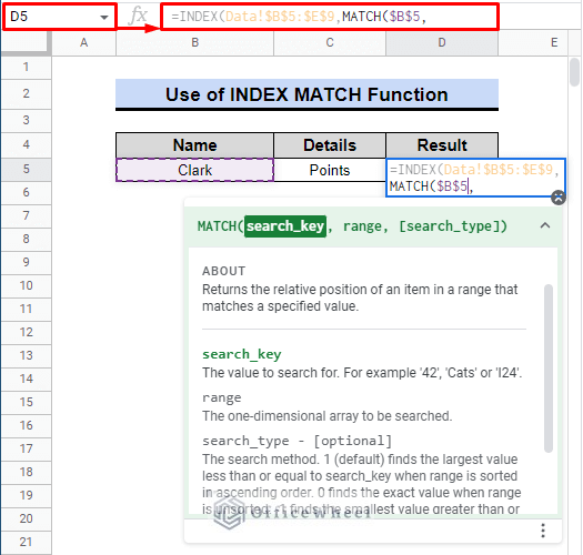
• After that, we must choose the range to search within. For example B5:B9.

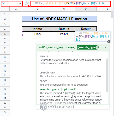
• Finally, we will use 0 at the conclusion because we want an exact match.

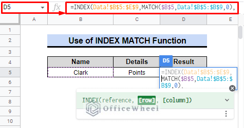
Step 3: Applying MATCH Function to Find Column Number

• To set the column value for the INDEX function using the MATCH function once more, we will follow the same procedure.
• The cell that will be compared in this instance is C5.
• The range of the column would therefore be B4:E4.
• For an exact match once more, we’ll choose 0.
• Final formula:

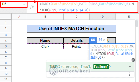
Step 4: Finalizing the Output

• Now, the formula will display the desired result if you press ENTER after it.

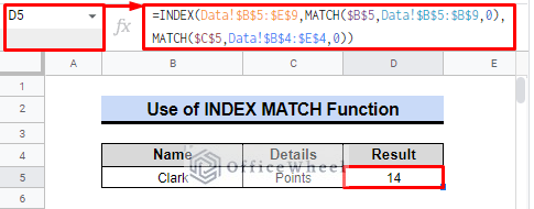
As you can see in the figure above, we searched for Clark and his points, and the INDEX MATCH function returned the value 14, which is what he received.

Similar Readings

• Google Sheets Conditional Formatting with INDEX-MATCH
• Google Sheets HLOOKUP to Return Column (3 Simple Ways)

Implementing Data Validation Tool in the Worksheet

Data validation is a strong tool that can assist you in maintaining clean and accurate data in your worksheets. To understand how to use Data validation with INDEX MATCH, look at the steps below.

Steps:

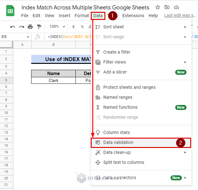
• Click Data > Data validation in the top menu from the Toolbar.

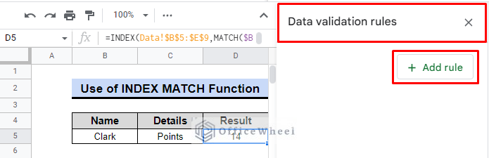
• In the data validation dialog box, Click “+ Add rule”.

• There will be a new dialog box. Choose where you wish to apply it in the range, for example, cell B5.
• Criteria > Drop Down (from a range)
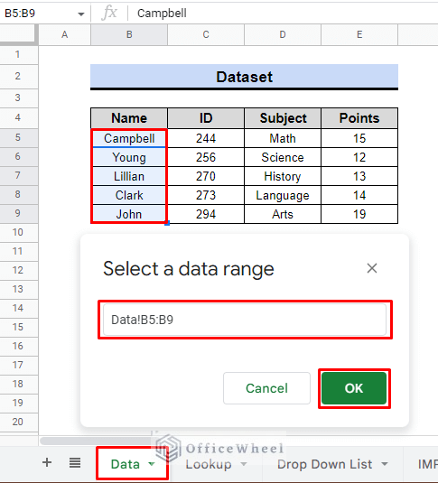
• Select the data range by selecting the box below afterward.

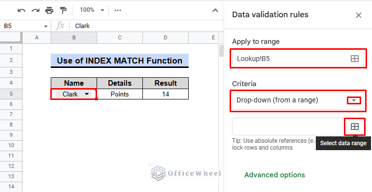
• For this example, the range should be from B5 to B9.
• Click OK to select the range.

• Then the following window will appear after selecting the range.

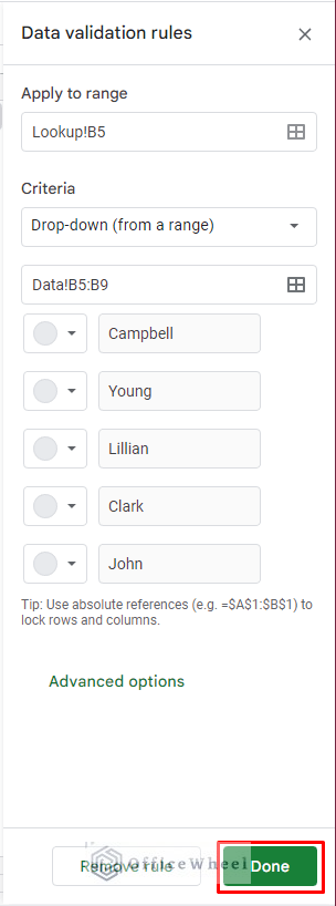
• Thereafter, click Done to see the drop-down menu.

• In cell C5, we can repeat the process to improve the INDEX MATCH function and search criteria.

Our search parameters can now be expanded with the aid of a drop-down menu, allowing us to quickly obtain any information.

Read More: How to Create Conditional Drop Down List in Google Sheets

How to Use IMPORTRANGE Function to Import Data from a Different Google Sheets

Assume that the source data is located in a different spreadsheet. You can import data from one spreadsheet into another in Google Sheets using the IMPORTRANGE function. We must employ the IMPORTRANGE function to use the data from that spreadsheet.

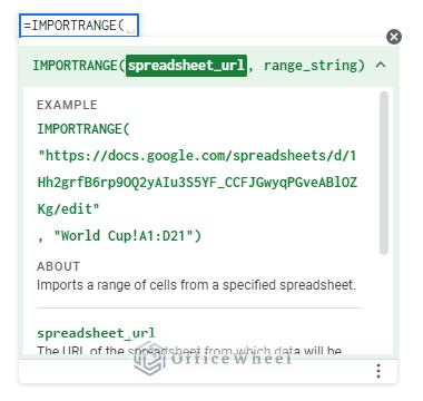
From the spreadsheet, we will need two items. The spreadsheet link or URL is one, while the cell range is another. With the help of the previous example, we will demonstrate the use of the IMPORTRANGE function.

Steps:

• We must copy the URL or link to the source article. We’ll also need it to verify the column and row for references.

• We will use the following formula as the cell reference for the INDEX function in cell D5.

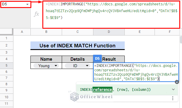
• Utilizing the MATCH function, we will set row values as follows:

• Once more, we must use the following formula to set the column values. The final formula is:

• Press ENTER to see the result.

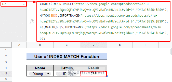
As you can see, using the IMPORTRANGE function, we were still able to obtain a similar result even if the original data was in a different sheet. We can also search for data in the source spreadsheet using the drop-down list.

What Makes INDEX MATCH Better than VLOOKUP in Google Sheets?

• Lookup Range:
  In contrast to VLOOKUP, which can only utilize a single range for both the lookup and return ranges, INDEX MATCH lets you specify independent lookup and return ranges.
• Column Reference:
  With INDEX MATCH, you can specify the column number of the cell you want to return as an optional argument in the MATCH function, which allows you to return a value from a specific column in the return range. With VLOOKUP, you must specify the column number as a fixed argument in the function, which means you can only return a value from a specific column.
• Lookup Type:
  Both INDEX MATCH and VLOOKUP allow you to specify the type of match you want to use, but INDEX MATCH provides more options for the match type.
• Performance:
  In general, INDEX MATCH outperforms VLOOKUP in terms of speed and effectiveness, especially when dealing with huge data sets. This is because INDEX MATCH may use the MATCH function to rapidly find the row or column having the match while VLOOKUP must search across the complete lookup range to get a match.

Read More: Combine VLOOKUP and HLOOKUP Functions in Google Sheets

Conclusion

One of the best parts about using INDEX MATCH across multiple sheets in Google Sheets is the ability to create a dynamic link between these sheets. This can save a lot of time and effort, as you don’t have to manually update the data in the destination sheet every time the source data changes. Overall, INDEX MATCH is not only a powerful but also a versatile tool for working with data in Google Sheets. Check OfficeWheel for more relevant content.

Related Articles

• [Fixed!] INDEX MATCH Is Not Working in Google Sheets (5 Fixes)
• How to VLOOKUP Left in Google Sheets (4 Simple Ways)
• How to Create Dependent Drop Down List in Google Sheets
• Match Multiple Values in Google Sheets (An Easy Guide)
• Match from Multiple Columns in Google Sheets (2 Ways)
• INDEX-MATCH with Multiple Criteria in Google Sheets (Easy Guide)
• Using INDEX MATCH in Google Sheets – A Deep Dive