While working on a dataset sometime we need the same value from other cells or another sheet, sometimes we need to know the exact place of a particular character. In that case, matching every character manually or checking the character’s position every time is time-consuming and tiring work. We can use different types of formulas and functions to make this work easier. In this article, We will learn how to return an exact match in Google Sheets using some practical examples.
A Sample of Practice Spreadsheet
You may copy the spreadsheet below and practice by yourself.
7 Suitable Ways to Return Exact Match in Google Sheets
The Dataset below contains Student Name and Total Marks. Here, we will show 7 practical yet simple examples to return an exact match in Google Sheets.
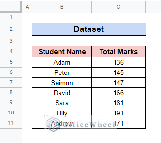
Suppose we want to lookup for an exact match to the student’s name and return the corresponding total marks. Follow the methods below to do that.
1. Using VLOOKUP Function
Now we will use the VLOOKUP function to return an exact match in Google Sheets using the following dataset. So, let’s start.
📌 Steps:
- First, select cell F5 to execute the VLOOKUP function.
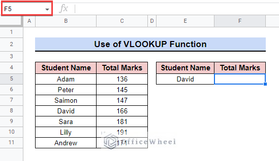
- Then enter =VLOOKUP( into the cell and click on cell E5 as the lookup value.
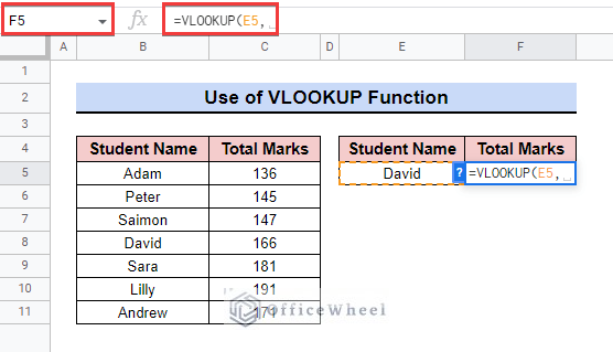
- After that, enter the range B5:C11 to extract the match value from the particular range.
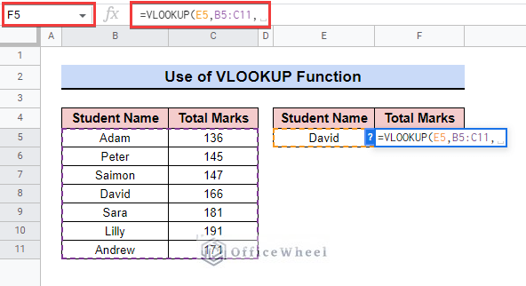
- Now, manually write 2 to get the value from the second column of the range and at last terminate the function with 0 or FALSE to get the exact value.
=VLOOKUP(E5,B5:C11,2,0)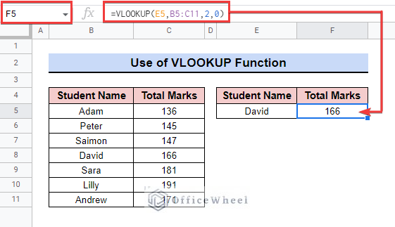
2. Applying XLOOKUP Function
Here, we will apply the XLOOKUP function to return the exact match in google sheets using the following dataset. So, follow the steps below.
📌 Steps:
- First, select cell F5 to execute the formula.
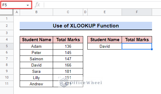
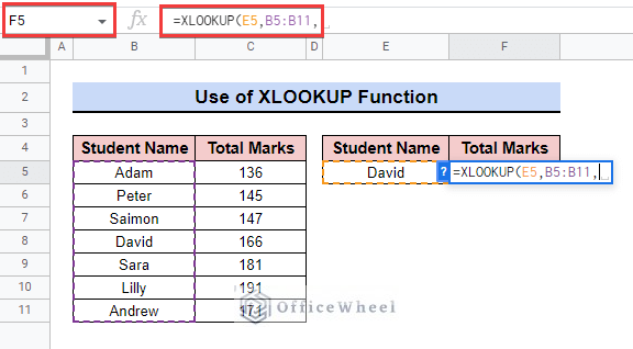
- Then, enter =XLOOKUP( using the lookup value in cell E5 and the lookup range as B5:B11 as below.
- After that, select the result range C5:C11 and write Null manually so that if the value doesn’t match it can return as null.
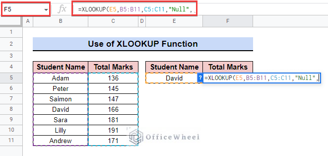
- Now, locate the position of the value to get the exact return from the formula as below.
=XLOOKUP(E5,B5:B11,C5:C11,"Null",2,-1)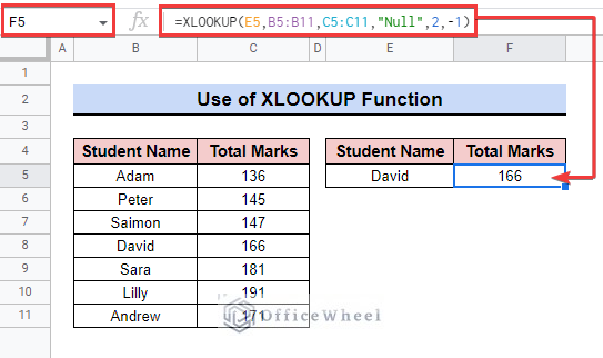
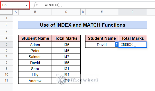
3. Utilizing INDEX and MATCH Functions
Here, we will utilize INDEX and MATCH functions to return the exact match in Google Sheets using the same dataset as before.
📌 Steps:
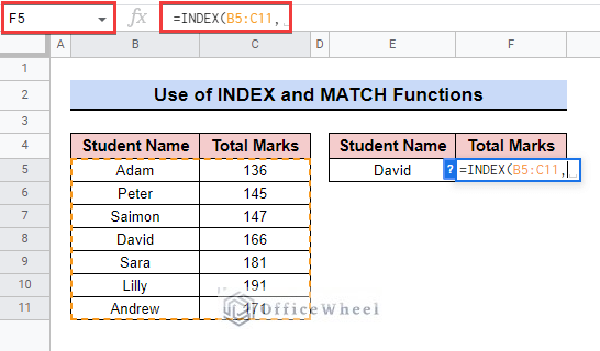
- First, select cell F5 to execute the formula and insert the INDEX function.
- Then, enter the lookup range B5:C11 to shortlist the area of the match.
- After that, enter the MATCH function and select lookup value cell E5.
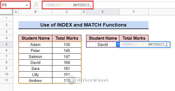
- Now, select the result range B5:B11 and end the range with 0 to close the range within column B.
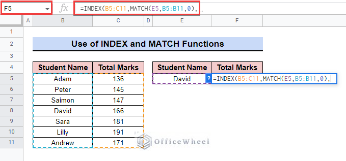
- At last, complete the formula with 2 to get the exact return from the second column of the lookup range.
=INDEX(B5:C11,MATCH(E5,B5:B11,0),2)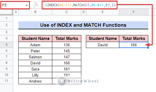
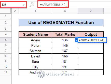
4. Executing REGEXMATCH Function
Here, we will execute the REGEXMATCH function to return the exact match in google sheets using the same dataset as before.
📌 Steps:
- First, select cell D5 and enter the ARRAYFORMULA function so that the output gets returned in an array.
- Then enter the REGEXMATCH function and select result range B5:B11 to get the value from the exact range.
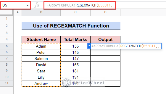
- After that, use ^David$ to return TRUE for an exact match to David from the dataset and the rest values will appear as FALSE as below.
=ARRAYFORMULA(REGEXMATCH(B5:B11,"^David$"))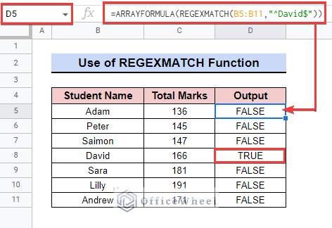
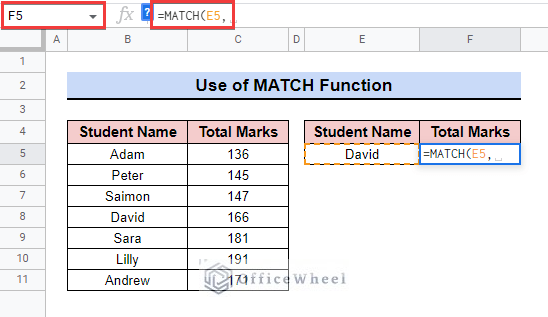
5. Using Basic MATCH Function
Now, we will execute the MATCH function to return the row number of the exact match from the other dataset in Google Sheets using the same dataset as before.
📌 Steps:
- First, select cell F5 and enter the function using cell C5 as the lookup value.
- Now, select the lookup range B5:B11 and complete the function with 0 to get the exact match. The formula will return the row number for the exact match.
=MATCH(E5,B5:B11,0)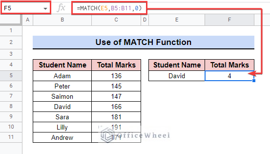
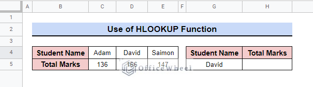
6. Applying the HLOOKUP Function
Here, we will apply the HLOOKUP function to return the exact match in google sheets using another dataset below. This dataset contains Student Name and Total Number.
📌 Steps:
- First, select cell F5 to execute the HLOOKUP function.
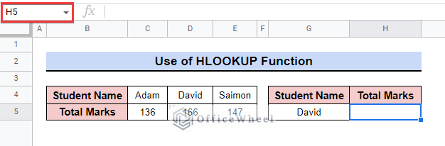
- Then enter =HLOOKUP( into the cell using the lookup value in cell G5.
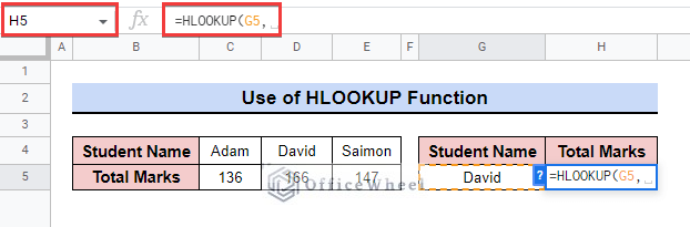
- After that, enter the range C4:E5 to extract the match value from the particular range.
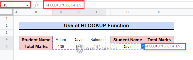
- Now, manually write 2 to get the value from the second column of the range, and at last complete the formula with 0 or FALSE to get the exact value.
=HLOOKUP(G5,C4:E5,2,0)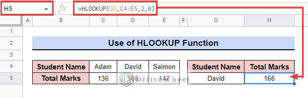
7. Using Find and Replace Tool
Here, we will use the Find and Replace tool to return the exact match in google sheets using the same dataset as before.
📌 Steps:
- First, select the lookup range B5:C11 and press Ctrl + H. Then the Find and Replace window will pop up as below.
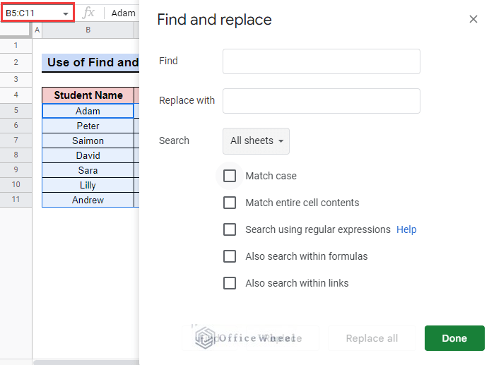
- Now Manually write David into the Find box as the lookup value is David.
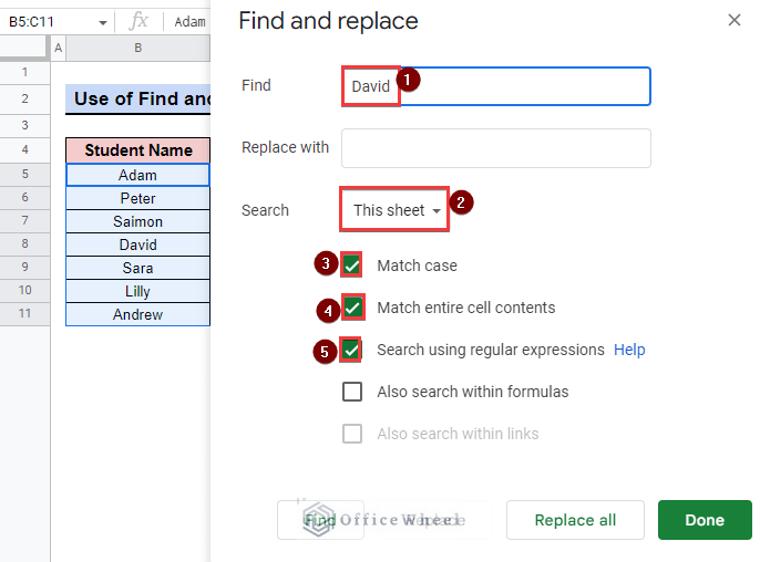
- After that, select This sheet in the Search criteria to search within the active sheet only. Next, select Match case, Match entire cell contents and Search using regular expressions to get the exact match as a return.
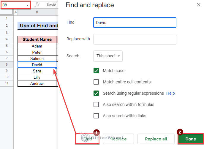
- Then, click the Find option and the search value will appear as the final output.
Things to Remember
- Use the ARRAYFORMULA function while executing the exact match with the REGEXMATCH function.
- Basic MATCH function will return to the position of the exact match, Match function doesn’t return to the value.
Conclusion
In this article, we explained how to return an exact match in Google Sheets with simple and practical examples. Hopefully, the examples will help you to apply this method to your own dataset. Please let us know in the comment section if you have any further queries or suggestions. You may also visit our OfficeWheel blog to explore more Google Sheets-related articles.