While working on a dataset sometimes we need to extract some specific data from that dataset but getting the data manually is difficult and time-consuming. It would be much easier to apply the INDEX function for a better solution. In this article, we will learn how to use the INDEX function in google sheets.
A Sample of Practice Spreadsheet
You may copy the spreadsheet below and practice by yourself.
What Is INDEX Function in Google Sheets?
The INDEX function returns a particular value from specific rows and columns of a dataset. For example, if you have a dataset with 10 names you will get particular data according to the condition.
Syntax
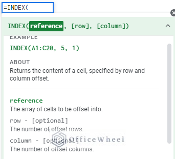
Arguments
| ARGUMENT | REQUIREMENT | Sample heading |
|---|---|---|
| reference | Required | Reference works as an array and combined the value. |
| row | Optional | The number of offset rows. |
| column | Optional | The number of offset columns. |
Return Value
Returns the value from a cell specified by the row and column numbers.
4 Easy Examples to Use INDEX Function in Google Sheets
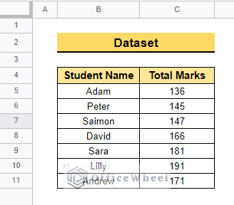
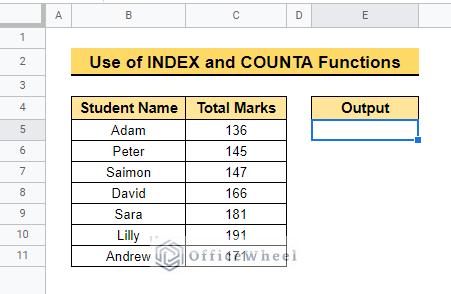
Now, the below dataset contains Student Name and Total Marks. Now we will use 4 different examples to show you how to use the INDEX function in Google Sheets.
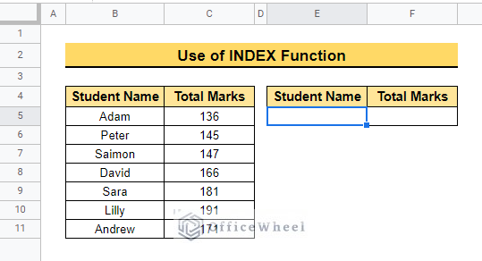
1. Using Basic INDEX Function
Here, we will show you the basic application of the INDEX function in Google Sheets.
📌 Steps:
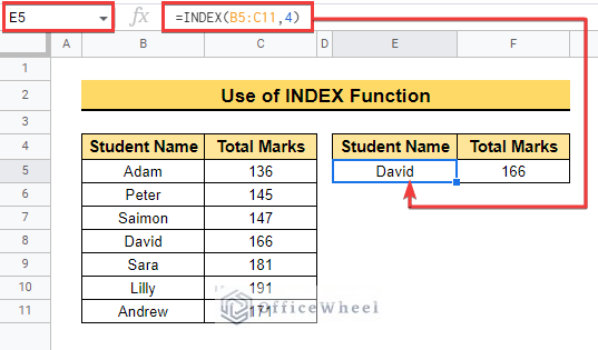
- First, select cell E5 to execute the formula.
- Then, type =INDEX( followed by range B5:C1 as the reference argument. Next type 4 to return the 4th row from the reference data range as follows.
=INDEX(B5:C11,4)
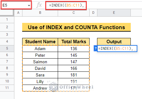
2. Applying INDEX and COUNTA Functions
Here, we will execute how to use the INDEX function with the COUNTA function.
📌 Steps:
- First, select cell E5 to execute the function.
- Then, enter the INDEX function and select the range B5:C11 as below.
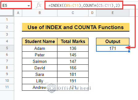
- After that, enter the COUNTA function to count the range C5:C11. The output of this function will be the row argument of the INDEX function. As a result, the formula will return the last value from the reference dataset.
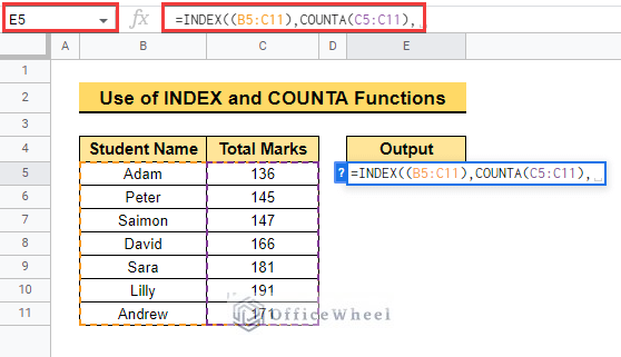
- Write 2 manually after finishing the function to get the last value of total marks. And the final output will be as below.
=INDEX((B5:C11),COUNTA(C5:C11),2)
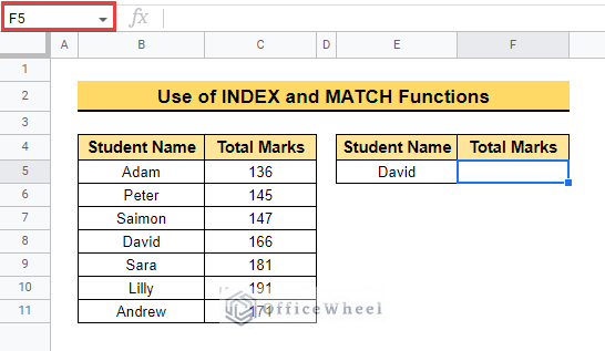
3. Combining INDEX and MATCH Functions
Here, we will use the INDEX function combined with the MATCH function for vertical lookup in Google Sheets.
📌 Steps:
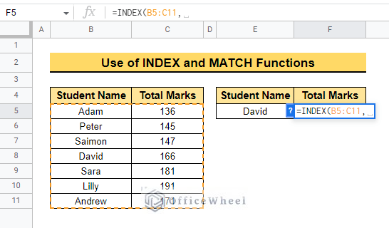
- First, select cell F5 to execute the formula as before.
- Then enter the function using the range B5:C11 as before.
- After that enter the MATCH function and select the range B5:B11 and lookup value cell E5.
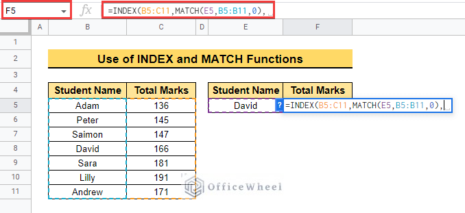
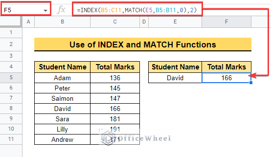
- At last, write 2 manually to get the value from the 2nd column of the range.
=INDEX(B5:C11,MATCH(E5,B5:B11,0),2)
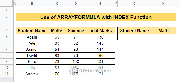
4. Utilizing ARRAYFORMULA with INDEX Function
We can also use the ARRAYFORMULA function with the different datasets below. The dataset below contains Student Name, Math, Science, and Total Marks. There we will find the exact output using the ARRAYFORMULA function both row-wise and column-wise.
4.1 Using the ARRAYFORMULA Function Row-wise
Here, we will extract the exact value of a row. For example, we want to extract Adam’s numbers. Now follow the steps below.
📌Steps:
- First, select cell G5 to execute the formula as before.
- Therefore, enter the ARRAYFORMULA function to return the output as an array.
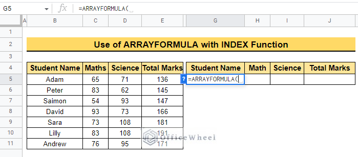
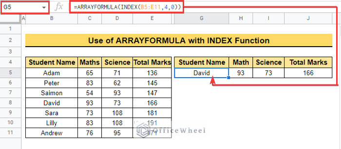
- Now enter the INDEX using the cell range B5:E11 and write 4,0 manually as a row will be extracted.
=ARRAYFORMULA(INDEX(B5:E11,4,0))
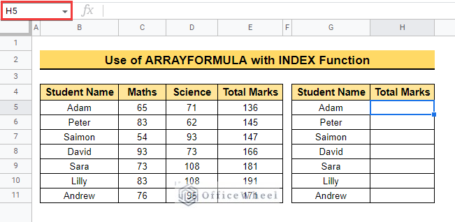
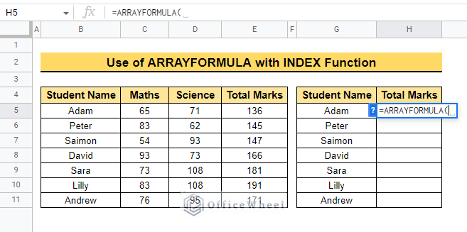
4.2.Executing ARRAYFORMULA Function Column-wise
Now, we will execute the exact value of a total column. For example, we will extract the total value of Math. Here, follow the steps below to execute this method.
📌Steps:
- Initially, select cell H5 to execute the formula.
- Moreover, enter the ARRAYFORMULA function to get the output as an array.
- After that, enter the INDEX function using the total cell range B5:E11 as below.
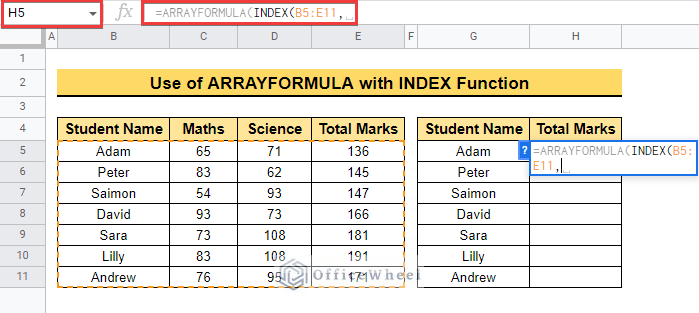
- Lastly, write 0, 4 manually as we will extract data from Total marks.
=ARRAYFORMULA(INDEX(B5:E11,0,4))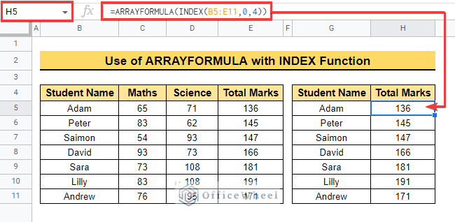
Alternative to INDEX Function in Google Sheets
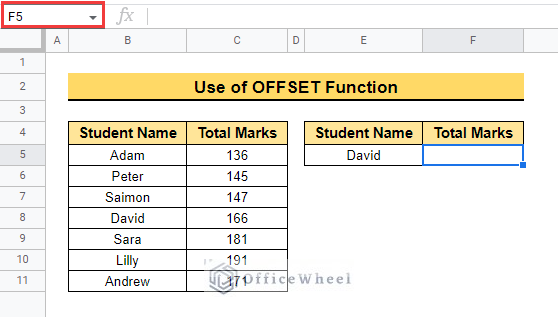
You can use the OFFSET function as an alternative to using the INDEX function in Google Sheets. Now follow the steps below to execute the formula.
📌 Steps:
- First, select cell F5 to execute the formula as below.
- Then enter the formula to get the value of the 3rd cell after cell C5 from column C. The final output will be as follows.
=OFFSET(C5,3,0)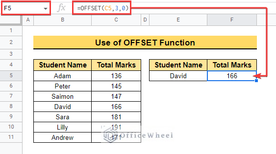
Things to Remember
- The INDEX function can be used individually and combined with other functions to get results.
- Always add the range of the INDEX function after finishing the function when the function is combined with the other function.
Conclusion
In this article, we explained the anatomy of the INDEX function. We also explained how to use the INDEX function in Google Sheets with simple examples. Hopefully, the examples will help you to apply this method to your own dataset. Please let us know in the comment section if you have any further queries or suggestions. You may also visit our OfficeWheel blog to explore more Google Sheets-related articles.