VLOOKUP with IMPORTRANGE Function in Google Sheets

Suppose you are working on two different spreadsheets at the same time. Now manually switching between the spreadsheets every time may become very time-consuming and difficult. It would be easier for you to look up all the data from one single spreadsheet. In this article, we will learn how to VLOOKUP from a different spreadsheet with the IMPORTRANGE function in Google Sheets.

A Sample of Practice Spreadsheet

You may copy the spreadsheet below and practice by yourself.

What Is IMPORTRANGE Function in Google Sheets?

The IMPORTRANGE function imports data within a particular range from a different spreadsheet using the spreadsheet URL and range string.

Syntax

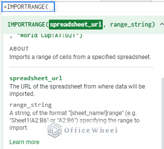
Argument

• spreadsheet_url: This is the URL of the source spreadsheet from which the data will be imported. This URL must be enclosed in double quotes. For example, suppose you want to import data from a spreadsheet called “Source”. Then you need to use the URL of this spreadsheet as “https://docs.google.com/spreadsheet/edit#1234″.
• range_string: Here, you input the range containing the required data within the source spreadsheet. For example: “‘Sheet1’! A2:D12”.

Return Value

• The final output will be the range selected from the other spreadsheet.

2 Examples of VLOOKUP with IMPORTRANGE Function in Google Sheets

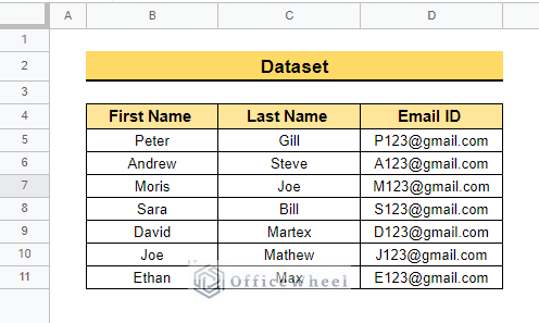
Here, the dataset below contains First Name, Last Name, and Email ID of some random people. Now, we will look up the Email ID from a different spreadsheet using the methods below. Let’s start.

1. Using VLOOKUP and IMPORTRANGE Functions

Here, we will apply the VLOOKUP and IMPORTRANGE functions to look up the First Name and return the Email ID from another spreadsheet. The steps are mentioned below.

📌 Steps:

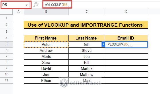
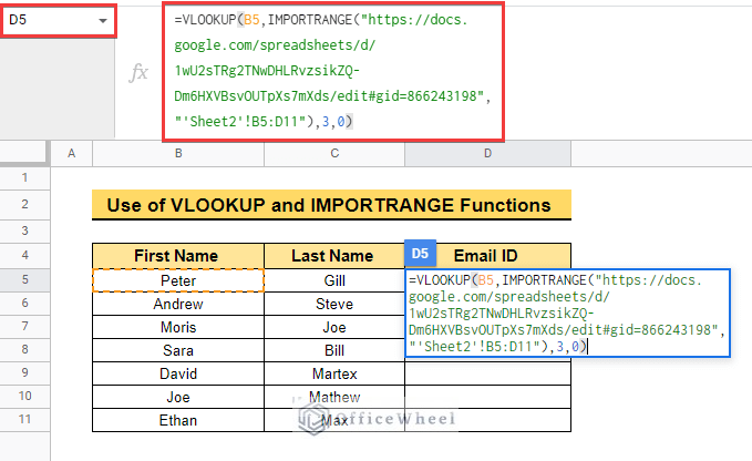
• First, select cell D5 and type =VLOOKUP( to insert the VLOOKUP function.
• Then select cell B5 to look up the value of that cell.

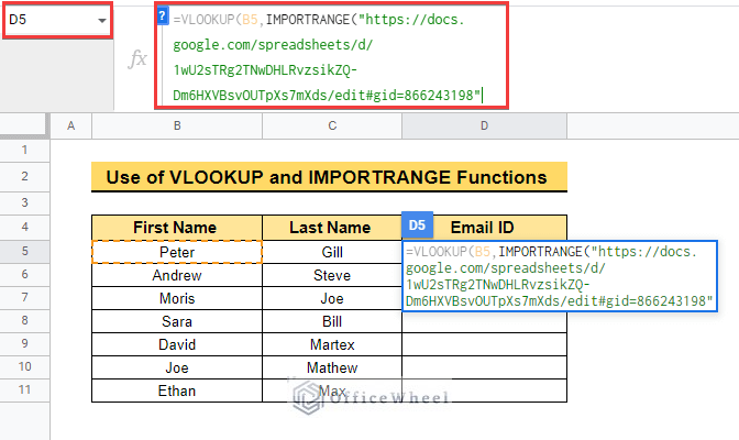
• Now, insert the IMPORTRANGE function and paste the URL of the source spreadsheet within double quotes as (“https://docs.google.com/spreadsheets/d/1wU2sTRg2TNwDHLRvzsikZQ-Dm6HXVBsvOUTpXs7mXds/edit#gid=866243198”).

• Then, write down the sheet name within single quotes, and put an exclamation mark (!) followed by the data range. Next, enclose the entire reference within double quotes as (“‘Sheet2’ !B5:D11”).

• After that, type 3 for the index and 0 for an exact match to complete the formula.

• Now, enter the formula and the final output will be as below.

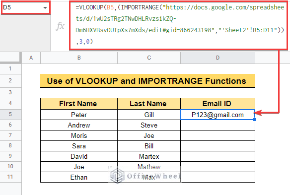
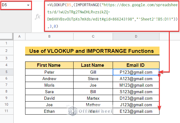
• At last drag down the fill handle and copy the same formula into the range D6:D11.

Read More: Google Sheets Vlookup Dynamic Range

Similar Readings

• How to Concatenate with VLOOKUP in Google Sheets
• Do Reverse VLOOKUP in Google Sheets (4 Useful Ways)
• How to Use VLOOKUP with IF Statement in Google Sheets
• VLOOKUP Multiple Columns in Google Sheets (3 Ways)
• How to Use VLOOKUP with Drop Down List in Google Sheets

2. Combining IFERROR, VLOOKUP, and IMPORTRANGE Functions

The VLOOKUP function will return an error in case it doesn’t find any matching result. Here we will combine the IFERROR function with the VLOOKUP and IMPORTRANGE functions to avoid that. The IFERROR function returns the specified output in case of errors. The steps are mentioned below.

📌 Steps:

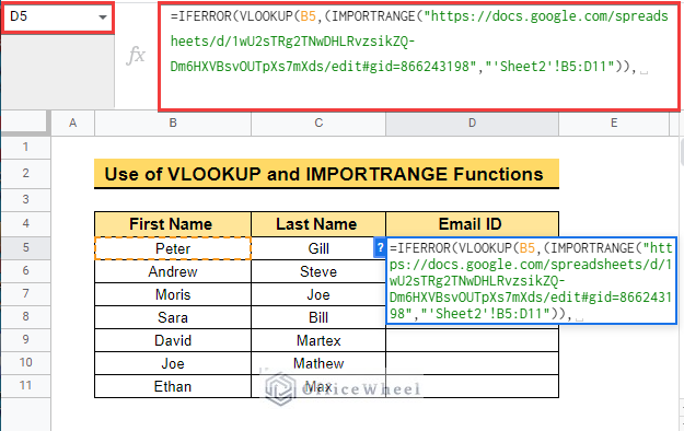
• First, select cell D5 and type =IFERROR( insert the IFERROR function.

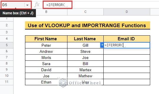
• Then, insert the VLOOKUP function as VLOOKUP(B5, where cell B5 contains the lookup value.

• Finally, enter the IMPORTRANGE function using the URL of the source spreadsheet within double quotes and then, write down the sheet name, and put an exclamation mark (!) followed by the data range. Then, write down the required range manually and keep this portion within another double quote as (“‘Sheet2’ !B5:B11”).as before.

• After that, type 3 for the index and 0 for an exact match. Then enter the formula to see the following result.

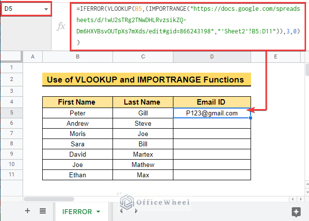
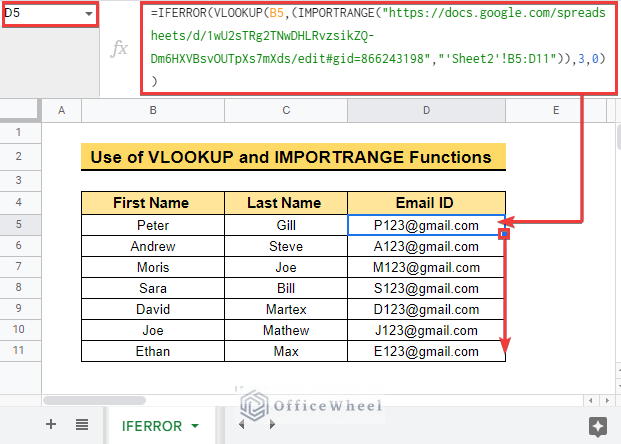
• Now, drag down the fill handle icon to see the same output as earlier.

Read More: How to Use IFERROR with VLOOKUP Function in Google Sheets

Alternative to Vlookup Using QUERY with IMPORTRANGE Function in Google Sheets

Using the VLOOKUP function to get the required data from another spreadsheet can be a difficult process sometimes. We can also use the QUERY function along with the IMPORTRANGE function to get the same result as obtained earlier. Follow the steps below to execute the formula.

📌 Steps:

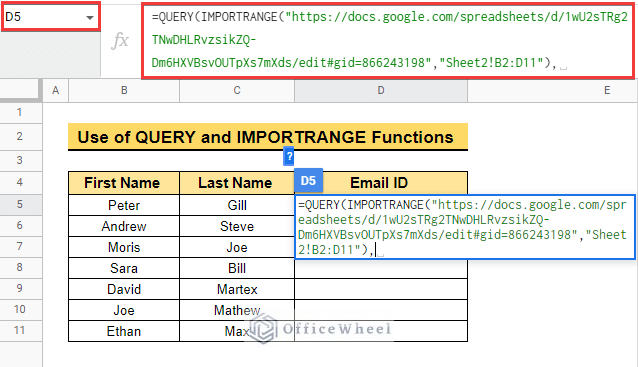
• First, Select cell D5 and insert the QUERY function.

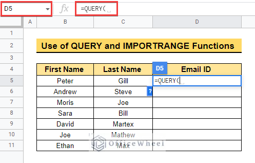
• After that, enter the IMPORTRANGE function using the URL of the source spreadsheet within double quotes and then, write down the sheet name, and put an exclamation mark (!) followed by the data range. Then, write down the required range manually and keep this portion within another double quote as (“‘Sheet2’ !B5:B11”) as before.

• After that, type “Select Col3 where Col1='”&B5&”‘” to complete the formula. This will allow you to copy the formula down. Now enter the formula to see the following result.

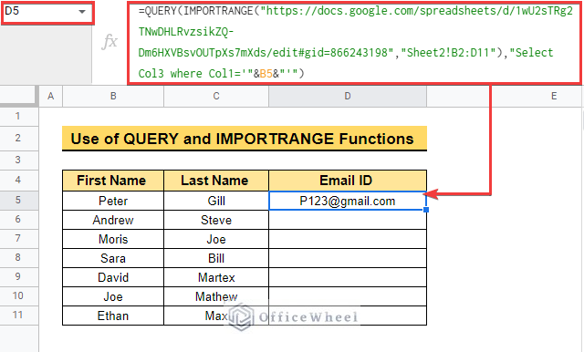
• Now, copy the formula down using the fill handle icon to get the final output as below.

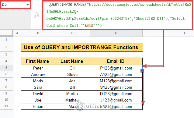
Read More: Alternative to Use VLOOKUP Function in Google Sheets

Things to Remember

• Always put the spreadsheet URL in a quotation to avoid errors while applying the formula.
• Always remember to add the sheet name while selecting the range.

Conclusion

In this article, we explained the anatomy of the IMPORTRANGE function. We also explained how to VLOOKUP with the IMPORTRANGE function in Google Sheets using different examples. Hopefully, the methods will help you to apply VLOOKUP with the IMPORTRANGE function to your own dataset. Please let us know in the comment section if you have any further queries or suggestions. You may also visit our OfficeWheel blog to explore more Google Sheets-related articles.

Related Articles

• How to Use Nested VLOOKUP in Google Sheets
• [Fixed!] Google Sheets If VLOOKUP Not Found (3 Suitable Solutions)
• How to VLOOKUP Between Two Google Sheets (2 Ideal Examples)
• Create Hyperlink to VLOOKUP Cell in Multiple Rows in Google Sheets
• How to VLOOKUP Last Match in Google Sheets (5 Simple Ways)
• Use VLOOKUP to Import from Another Workbook in Google Sheets
• How to Use VLOOKUP for Conditional Formatting in Google Sheets