In Google Sheets, if you want to track the position or serial of any specific value in a range, the MATCH function will be helpful. This article will show you how to use the MATCH function in Google Sheets.
A Sample of Practice Spreadsheet
You can download spreadsheets from here and practice.
What Is MATCH Function in Google Sheets?
The MATCH function is fairly basic in google sheets. It only returns the serial number, not the specific value. The search value can be a text, a number, or data.
Syntax
The following is the syntax for the MATCH function:
=MATCH(search_key, range, search_type)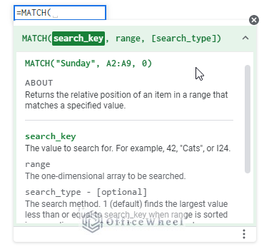
Arguments
The arguments of the MATCH function are as follows:
| ARGUMENT | REQUIREMENT | FUNCTION |
|---|---|---|
| search_key | Required | The specific value that you want to look up. |
| range | Required | A set of data whether a column or a row from where the specific value can look up. |
| search_type | Optional | It allows Google Sheets about the arrangement of the range to make the search faster.
1: applicable for the ascending order range 0: applicable for both sorted and unsorted data. -1: applicable for descending order range. |
Output
The formula =MATCH(“Robert”,C5:C9,0) will look for the relative position of the text value, and it returns ‘3’ as output which means the value is in the third cell of the range.
2 Suitable Scenarios to Use MATCH Function in Google Sheets
You can look up the position of any specific value from both sorted and unsorted data ranges.
1. Working with Unsorted Data
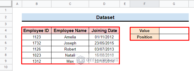
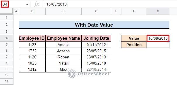
By inserting numeric, text, and date values in an unsorted data range, you can easily locate the relative position of the desired value. Here, we develop a dataset containing Employee ID, Employee Name, and Joining Date. We also create a value cell where you put your search key and can apply the MATCH function in the position cell to find the position of the value.
1.1 With Numeric Value
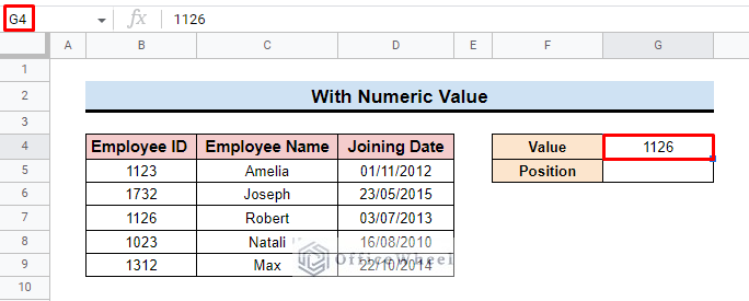
If you want to find the location of a numeric value,
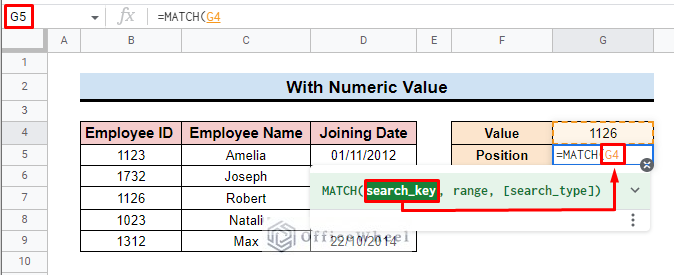
- First, insert a numeric value for the search key. Here we input employee ID 1126 as our search key.
- Now in the position cell apply the MATCH function.
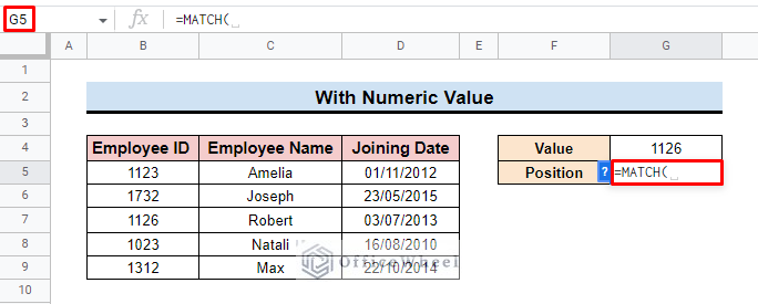
- Insert the G4 cell as the first argument of the function.
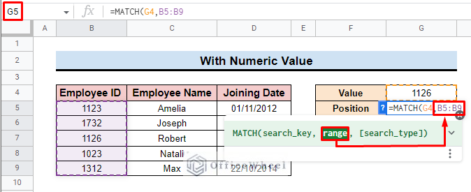
- After that add the range in the function. Here, we insert the entire Employee ID column as a range.
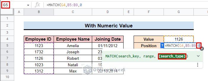
- As search_type we add “0” to get the correct result. It is because of the unsorted nature of the data range.
- Finally, press ENTER and you will find the position of your desired value in the data range.
=MATCH(G4,B5:B9,0)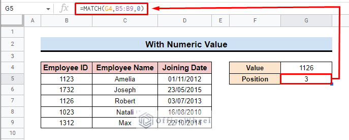
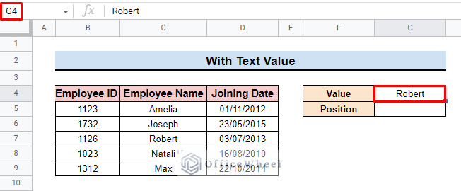
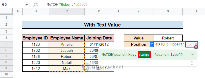
1.2 With Text Value
You can also search for text value positions in the dataset. To do so,
- First, input a text value for which position you want to search. Here we insert the employee’s name” Robert”.
- Then apply the MATCH function in cell G5.
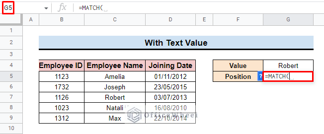
- Now, add the G4 cell as the first parameter of the function.
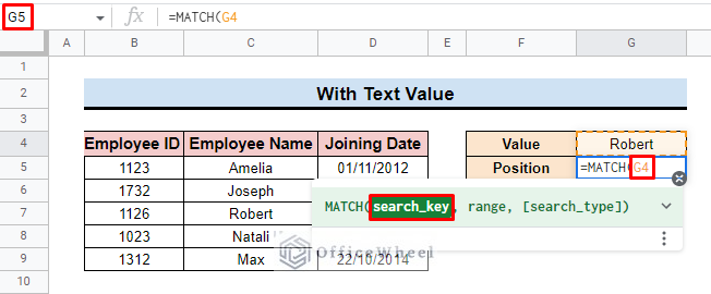
- Instead of a cell, you can also input the text value directly. Here, we add “Robert” as search_key.
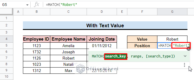
- After that insert the range. We add C5:C9 for the range parameter.
- At the end, add 0 to achieve the exact result.
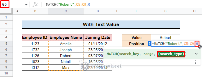
- Finally, press ENTER and you will get the relative position of the text value “Robert” in the range.
=MATCH(“Robert”,C5:C9,0)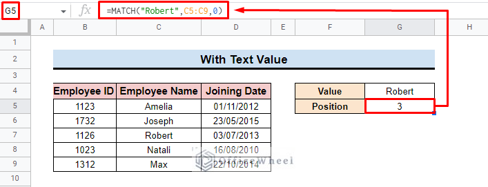
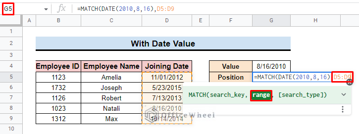
1.3 With Date Value
If you insert a date in your dataset you can apply the DATE function. The syntax for the function is:
=DATE(year,month,day)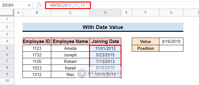
To apply the MATCH function for date value,
- At first, add a date value for which position you want to track.
- Then apply the MATCH function in cell G5.
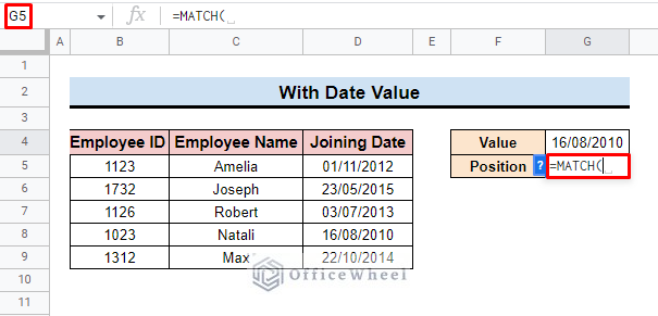
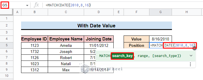
- Now enter the DATE function as search_key.
- Alternatively, you can also input the cell G4 as search_key, which contains the required date.
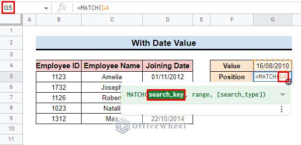
- After that, insert the range for the function. Here, we add the Joining Date column.
- In the end, input 0 to get the exact result.
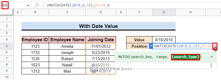
- Finally, press ENTER and the relative position of the desired text is shown in the selected cell.
=MATCH(DATE(2010,8,16),D5:D9,0)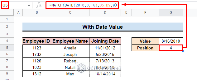
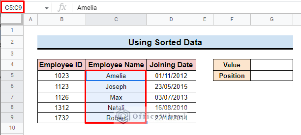
2. Using Sorted Data
To look up relative position of the desired value, you can also apply a sorted data range for the MATCH function. For sorted data, in MATCH function you can use 1 or -1 along with 0 as the search_type parameter to get the exact result. Here, 1 is for ascending order data range and -1 is for descending order data range. So,
- First, sort the range from where you want to know the relative position of your desired value. Ignore this if you already have a sorted dataset.
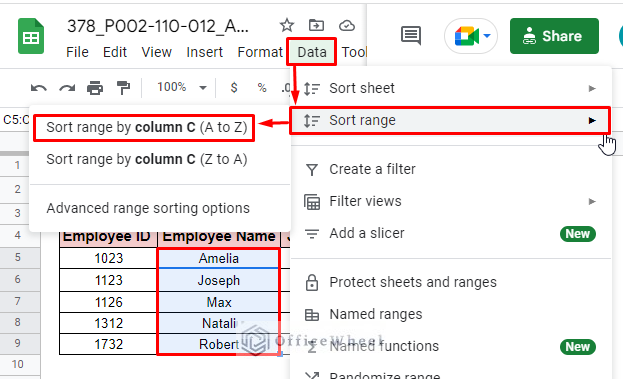
- Here is the sorted form of the selected data range. Since it is text, it was sorted in alphabetical order.
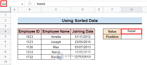
- Now, add a value in cell G4 to find its relative position.
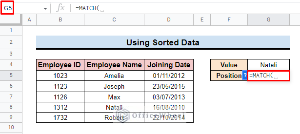
- After that, in cell G5 insert the MATCH function.
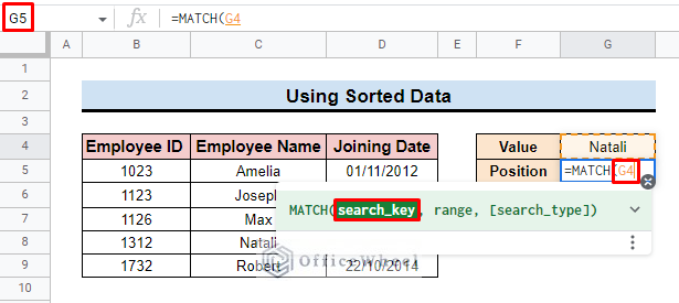
- Add the G4 cell as a search key.
- Then select the entire Employee Name column as a range which is C5:C9.
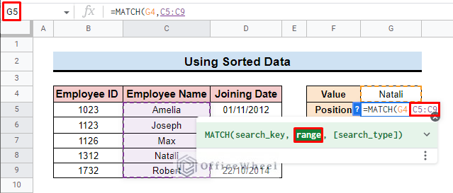
- In the end, insert 1 as search_type. Here we use the ascending order of the range so that we will get the exact value by adding 1 instead of 0.
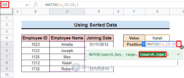
- Finally, press Enter and you will get the exact relative position of the selected value.
=MATCH(G4,C5:C9,1)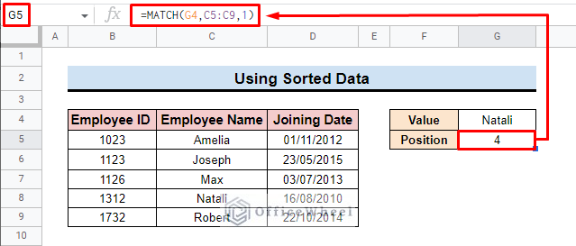
How to Use Combined INDEX MATCH Formula in Google Sheets
Though the MATCH function is a basic function, the combination of INDEX and MATCH functions is very powerful in Google Sheets. The INDEX MATCH function is considered the alternative to the VLOOKUP function and can solve many problems of lookup values.
The syntax of the INDEX function is as follows:
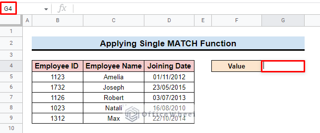
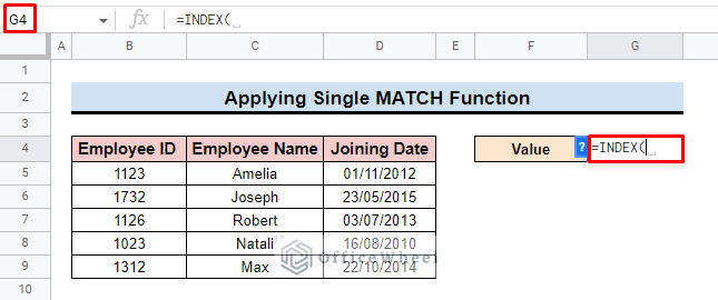
=INDEX(reference, row, column)1. Single MATCH Function
To apply the INDEX MATCH function for single criteria,
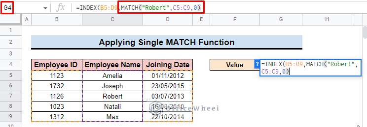
- First, select the value cell G4 to apply the formula.
- Then apply the INDEX function.
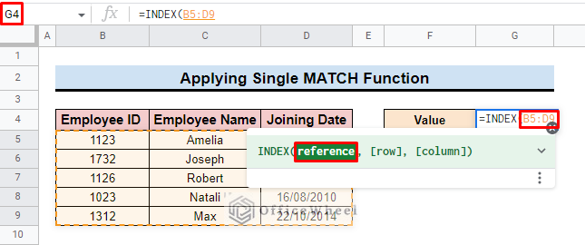
- After that add the range for the function. Here, we add the entire dataset as a range.
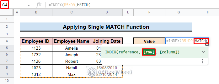
- Now as a row parameter, add the MATCH function.
- Then insert the search key for the MATCH function. Here we add “Robert” as a search key.
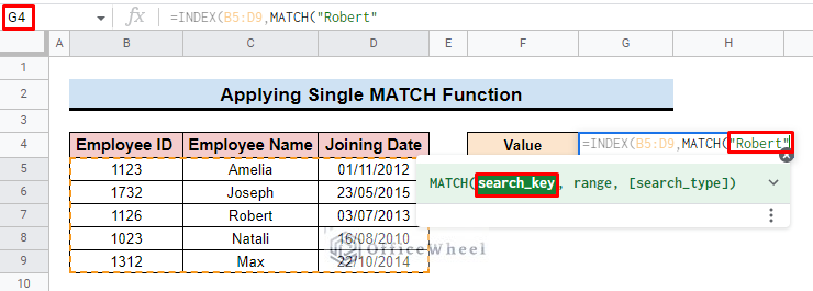
- Add the entire Employee Name column as a range. And input 0. Close the bracket to finish the MATCH function.
- After that, add the column number for the INDEX function. Here, we add 1 which represents the Employee ID column.
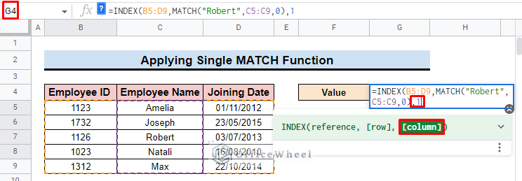
- Finally, press ENTER and you will find the employee ID for the employee “Robert”.
=INDEX(B5:D9,MATCH(“Robert”,C5:C9,0),1)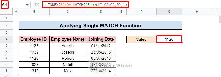
Read More: How to Return Exact Match in Google Sheets (7 Suitable Ways)
2. Multiple MATCH Functions
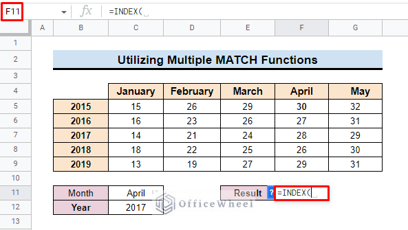
We can also use multiple MATCH functions along with the INDEX function to find out desired value from complex or large datasets. To show this, we create a dataset representing monthly temperatures for different years. Here, we want to look up April 2017 temperature value.
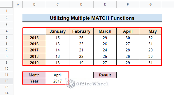
- So, first, insert the INDEX function in cell F11.
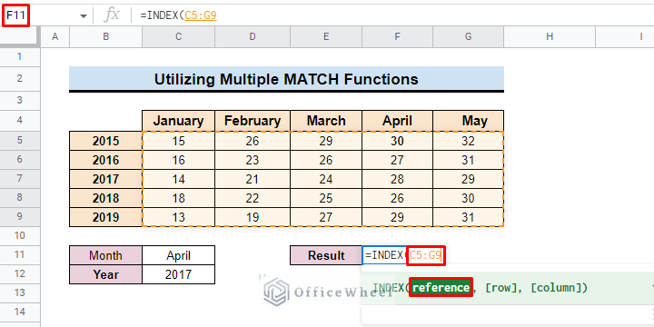
- Then insert the entire dataset as a reference. Here we add C5:G9 as a reference.
- Now, as the row value applies the first MATCH function where C12 is the search_key, B5:B9 represents the range and FALSE is set for getting the exact value.
MATCH(C12,B5:B9,FALSE)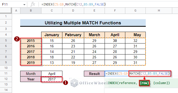
- After that, as column value apply another MATCH function where C11 represents the search_key, C4:G4 is the range, and FALSE is set to get an accurate result.
MATCH(C11,C4:G4,FALSE)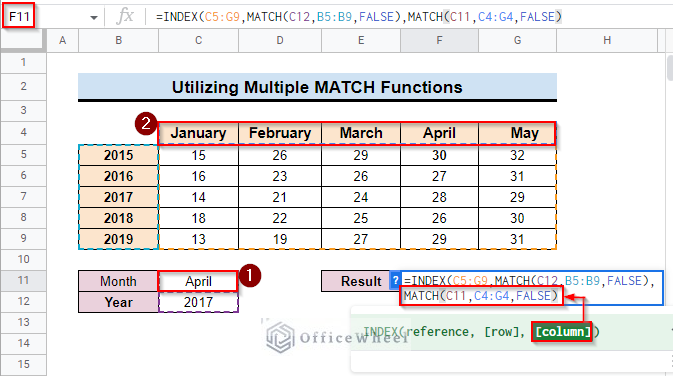
- Finally, press ENTER and you will find the desired value in the selected cell.
=INDEX(C5:G9,MATCH(C12,B5:B9,FALSE),MATCH(C11,C4:G4,FALSE))Read More: How to Match Cells Between Two Columns in Google Sheets (6 Ideal Methods)
How to Solve ‘MATCH Function Not Working?’ in Google Sheets
- Ensure Exact Match: You have to be careful about the exact match of the function. for instance, you will get the exact result when you add 0 for both the sorted and unsorted ranges.
- Insert Proper Range: You have to choose the correct range to run the function properly.
- Conscious about Format Issue: You have to be conscious about the search_key formatting because if the formatting of the value that location you want to track is not matched with the search_key, then the function shows an error.
- Differentiate between Sorted and Unsorted Data: When you choose 0 for “search_type” you can use both sorted or unsorted data ranges. But you have to choose “1” for the ascending order range and “-1” for descending order range.
Conclusion
Hope that this article will help you to understand how to use the MATCH function in Google Sheets. To explore much deeper about different functions of Google Sheets you can visit the OfficeWheel website.