A dependent drop down list is used when one wants to show only relevant information for subsequent dropdowns. It is also known as a dynamic dropdown list. Here, we will discuss 4 useful methods of creating a dependent drop down list in Google Sheets.
A Sample of Practice Spreadsheet
You can get the Practice Workbook from here and practice independently.
4 Useful Methods to Create Dependent Drop Down Lists in Google Sheets
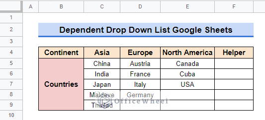
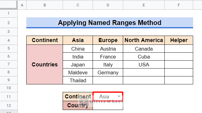
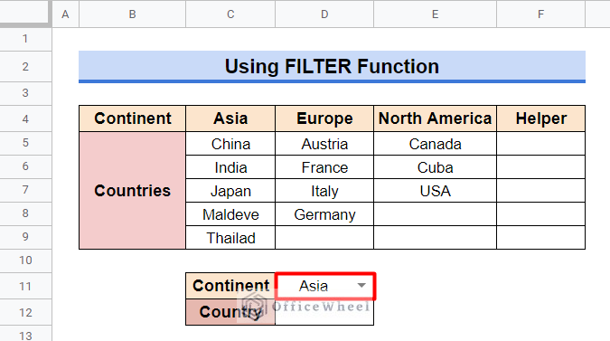
First of all, let’s get introduced to our data set which contains several continents and some of the countries in that continents. We have taken an additional column called “Helper” for calculation purposes.
1. Use ARRAYFORMULA Function in Google Sheets to Make a Dependent Drop Down List
In this method, we will use the ARRAYFORMULA function to create dependent dropdown lists. Firstly, we have to create a simple dropdown list using the Data Validation Tool. After that, using ARRAYFORMULA function and Data Validation Tool we will be able to create the dependent dropdown list.
Steps:
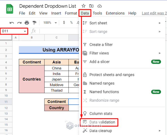
- Select Cell D11 (where you want to create the first dropdown list) and then go to the Data ribbon and click on Data Validation.
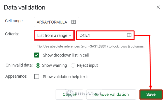
- In the popped-out window, set the List from a range as C4:E4 (Continent names) and then click on Save.
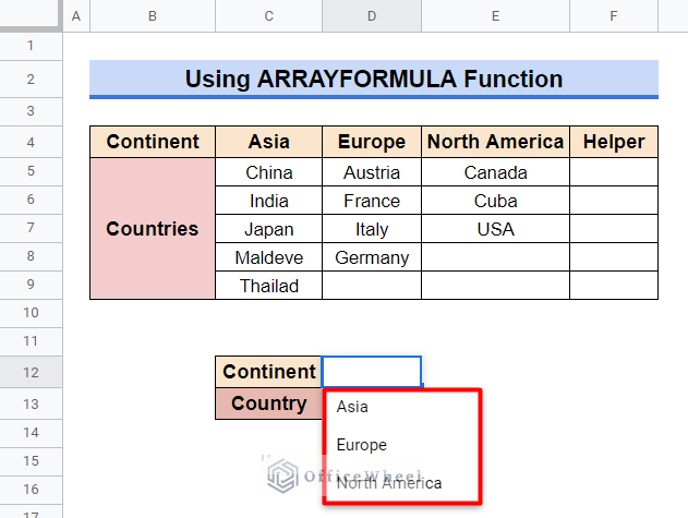
- At this point, the first dropdown list has been created. After clicking on the dropdown icon on that cell, you will get the dropdown list.
- Now, in Cell F5 (first row of the Helper column) type in the following formula and press Enter key.
=ARRAYFORMULA(IF(D11=C4,C5:C9,IF(D11=D4,D5:D8,E5:E7)))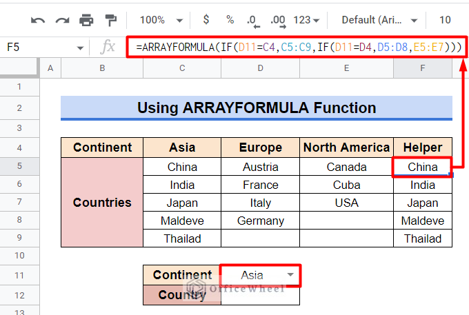
Formula Breakdown:
- IF(D11=D4,D5:D8,E5:E7)
The IF function returns the array D5:D8 when the criterion D11=D4 is TRUE and the array E5:E7 if the criterion is FALSE.
- ARRAYFORMULA(IF(D11=C4,C5:C9,IF(D11=D4,D5:D8,E5:E7)))
The ARRAYFORMULA function enables the display of the array returned by the nested IF function.
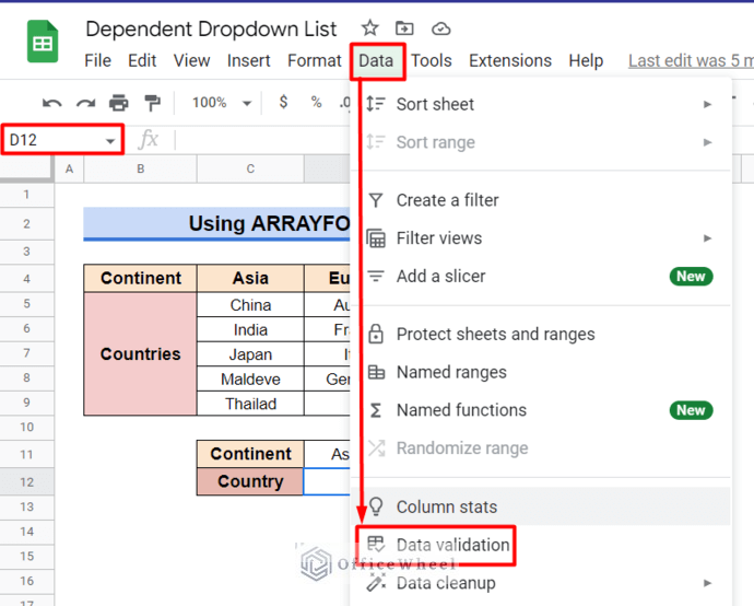
- After that, select Cell D12 (where you want to create the second dropdown list) and then go to the Data menu and click on Data Validation.
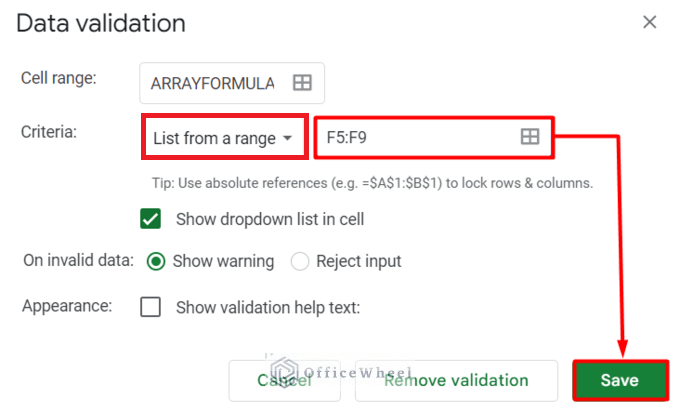
- In the popped-out window, set the List from a range as F5:F9 (Dependent country names) and then click on Save.
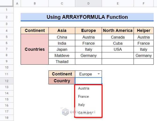
- The second dropdown list has now been created. After clicking on the dropdown icon on that cell, you will get the dropdown list.
Read More: How to Edit Data Validation in Google Sheets (With Easy Steps)
2. Apply the Named Ranges Method to Create Dependent Drop Down List in Google Sheets
In this method, we will use a combination of Named Ranges and the INDIRECT function to create a dependent drop down list in Google Sheets.
Steps:
- Use the first three steps from Method 1 to create a dropdown list in Cell D11.
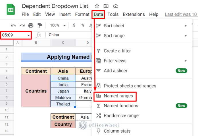
- Now, select Cells C5:C9, go to the Data ribbon, and click on Named Ranges.
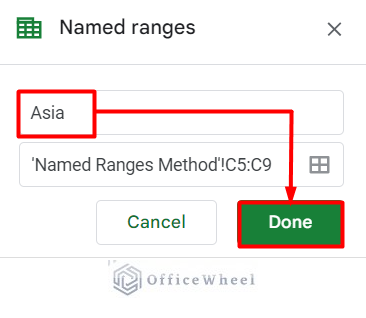
- In the popped-out window change the name to Asia and click on Done. (Note: If the name consists of multiple words, then use “_” between them. Example: North_America).
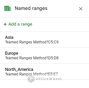
- Repeat the previous two steps for other Continents.
- Now, in Cell F5 type in the following formula and press Enter key.
=IF(D11=C4,INDIRECT("Asia"),IF(D11=D4,INDIRECT("Europe"),INDIRECT("North_America")))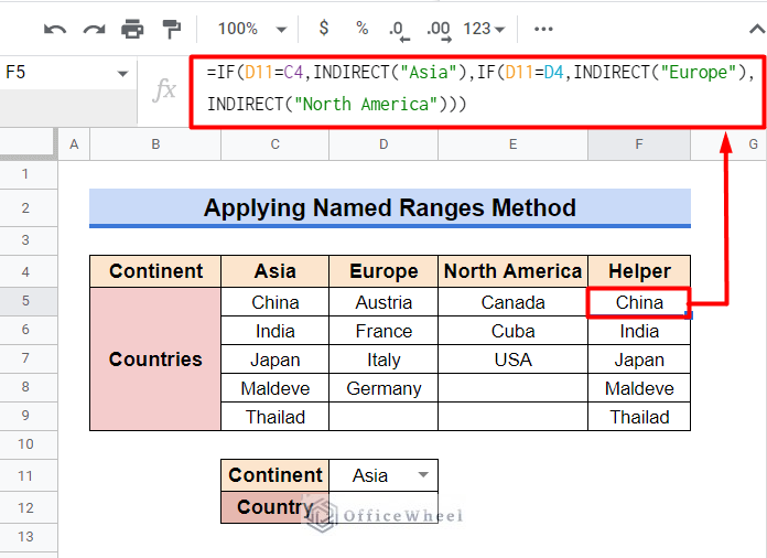
Formula Breakdown:
- INDIRECT(“Asia”)
The INDIRECT function returns the Named Range reference specified by the string “Asia”.
- IF(D11=C4,INDIRECT(“Asia”),IF(D11=D4,INDIRECT(“Europe”),INDIRECT(“North_America”)))
The IF function will INDIRECT one Named Range when the criterion for that Named Range is TRUE and the rest is FALSE.
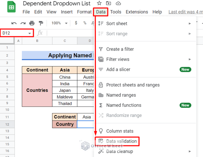
- After that, select Cell D12 (where you want to create the second dropdown list) and then go to the Data ribbon and click on Data Validation.
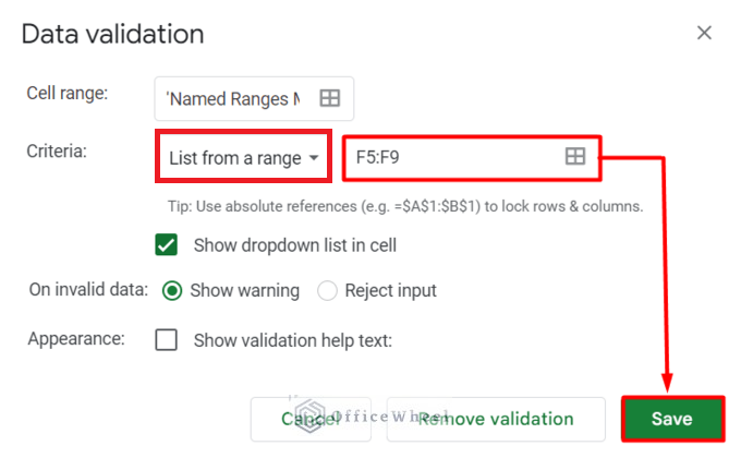
- In the popped-out window, set the List from a range as F5:F9 (dependent Country names) and then click on Save.
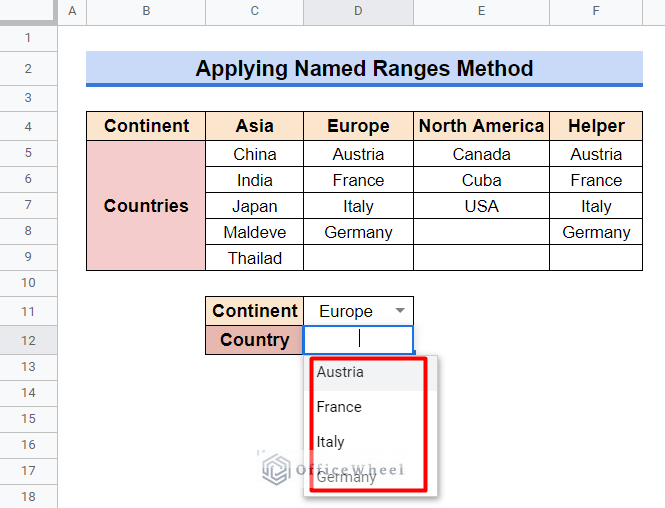
- The second dropdown list has now been created. After clicking on the dropdown icon on that cell, you will get the dropdown list.
Read More: Create Multiple Dependent Drop Down List in Google Sheets
Similar Readings
- How to Add Color to Drop Down List in Google Sheets (Easy Steps)
- Use VLOOKUP with Drop Down List in Google Sheets
- How To Lock Rows In Google Sheets (2 Easy Ways)
3. Use the FILTER Function in Google Sheets to Create Dependent Drop Down List
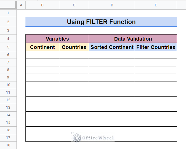
We will use the FILTER function to create the dependent drop down list in this method. We require two worksheets for this method (One to create the dropdown list and another to create a filter). It is mandatory that we save the worksheets as “FILTER Function” and “Filter Data Validation” respectively.
Steps:
- In the “FILTER Function” worksheet, use the first three steps from Method 1 to create a dropdown list in Cell D11.
- Now, in the “Filter Data Validation” worksheet, create a chart like the following.
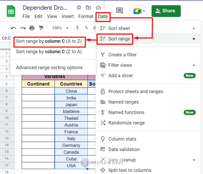
- Copy the Country names in Column C. Select Cells C6:C17 and go to the Data ribbon and click on Sort Range > Sort Range by Column C (A to Z).
- Manually input the name of the Continents for each country.
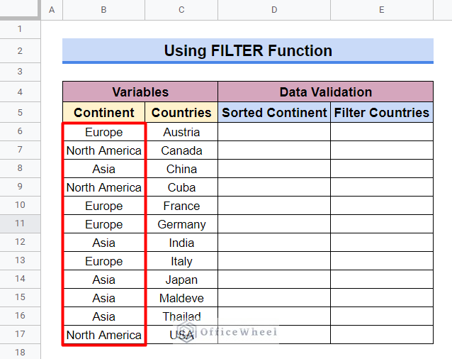
- Now, we will apply a combination of SORT and UNIQUE functions to sort Continents. For that, type the following formula in Cell D6 and press Enter key.
=SORT(UNIQUE(B6:B17),1,TRUE)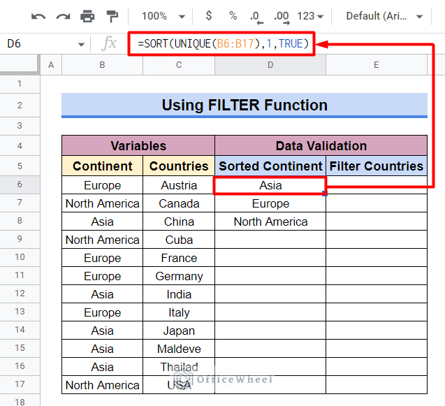
Formula Breakdown:
- UNIQUE(B6:B17)
The UNIQUE function will return unique rows in the B6:B17 range while discarding duplicates.
- SORT(UNIQUE(B6:B17),1,TRUE)
The SORT function will return the first n items after sorting them from the B6:B17 range.
- Now, in Cell E6, type the following formula and press Enter key.
=FILTER(C6:C17,B6:B17='FILTER Function'!D11)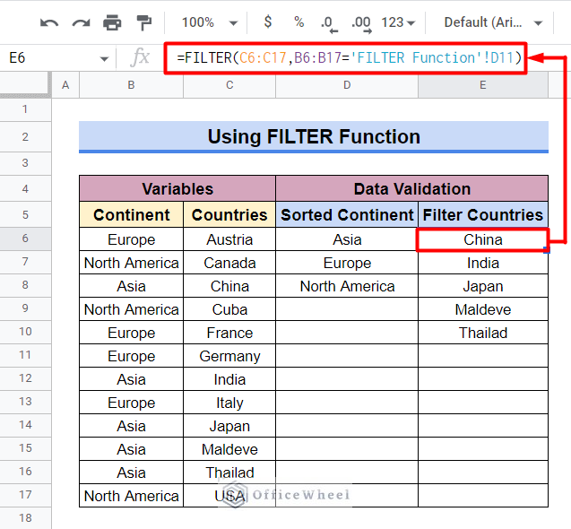
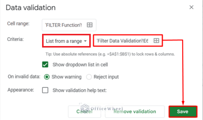
- Now, in the “FILTER Function” worksheet, select Cell D12, go to the Data ribbon, and click on Data Validation. In the popped-out window, set List from a range as ‘Filter Data Validation’!E6:E10 and then click on Save.
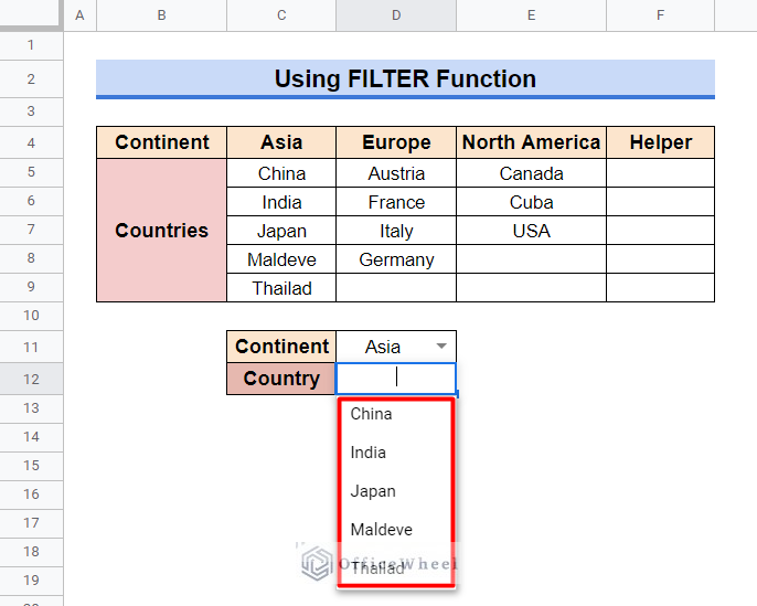
- The second dropdown list has now been created. After clicking on the dropdown icon on that cell, you will get the dropdown list.
Read More: How to Remove Data Validation in Google Sheets
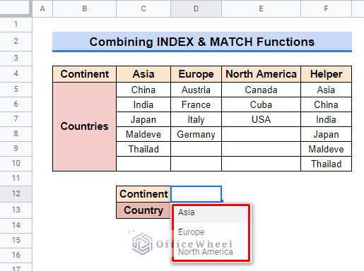
4. Combine INDEX and MATCH Functions to Create Dependent Drop Down Lists in Google Sheets
In our last method, we will combine the INDEX and MATCH functions to create a dependent drop down list in Google Sheets.
Steps:
- Use the first three steps from Method 1 to create a dropdown list in Cell D11.
- Now, in Cell F5, type the following formula and press Enter key.
=INDEX(C4:E9,,MATCH(D11,C4:E4,0))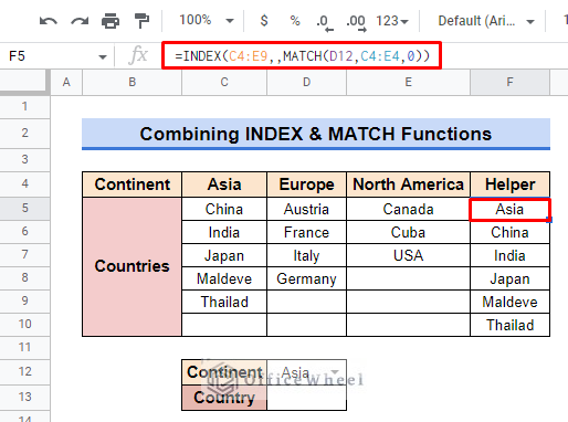
(Note: We have inserted a whole column as a single entity. So, in output with country names we also have continent names.)
Formula Breakdown:
- MATCH(D11,C4:E4,0)
The MATCH function will return the relative position of Cell D11 in array C4:E4. Here ‘0’ means exact match.
- INDEX(C4:E9,,MATCH(D11,C4:E4,0))
The INDEX function will return the content of the cell indicated by MATCH(D11,C4:E4,0) specified within array C4:E4.
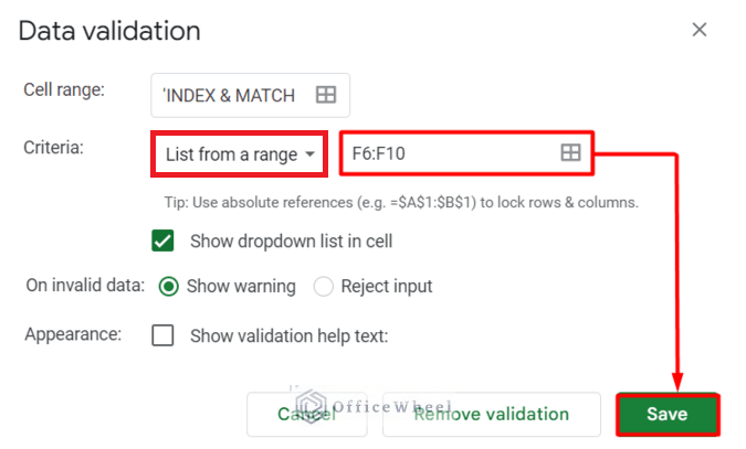
- Now, select Cell D12, go to the Data ribbon, and click on Data Validation. In the popped-out window, set List from a range as F6:F10 and then click on Save.
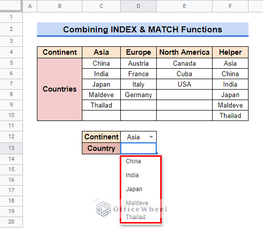
- The second drop-down list has now been created, After clicking on the dropdown icon on that cell, you will get the dropdown list.
Read More: How to Use Data Validation in Google Sheets from Another Sheet
Things to Be Considered
- Named Ranges do not accept Space between names. Hence, put a “_” between the names.
- In method 4, the entire column has been extracted as a single entity. Therefore, it contains the column heading. Remember to exclude it during Data Validation.
Conclusion
That concludes our article on how to create a dependent drop down list in Google Sheets. We hope the above methods were good enough for operations. Feel free to leave any queries or advice in the comment section.
Related Articles
- How to Insert a Drop-Down List in Google Sheets (2 Easy Ways)
- Create Drop Down List in Google Sheets from Another Sheet
- How to Edit Drop-Down List in Google Sheets
- Create Drop Down List for Multiple Selection in Google Sheets
- How to Create Conditional Drop Down List in Google Sheets
- Dependent Drop Down List for Entire Column in Google Sheets