Today, we will look at how to perform a match from multiple columns in Google Sheets. This process is useful if you want to extract values based on multiple criteria/column values.
2 Ways to Match from Multiple Columns in Google Sheets
1. Using INDEX MATCH to Match from Multiple Columns
The first method we will use is perhaps the most powerful in our article today, which is the INDEX-MATCH formula.
To show this method, we have the following worksheet:
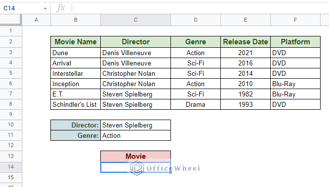
While this is just a part of a larger database, it contains various types of data. From here, we will be matching the Director name and Genre values from the column to retrieve the name of the Movie.
Our formula:
=INDEX(B3:B8,MATCH(1,(C3:C8=C10)*(D3:D8=C11),0))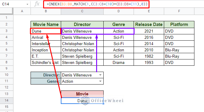
As you can see, we are combining the data from cells C10 and C11 as our match criteria from the table. The MATCH function within the formula returns the row index for the INDEX function to help retrieve the correct value.
However, we will be presented with an error if the formula is unable to find a correct match. So as a failsafe, we enclose this formula in the IFERROR function.
=IFERROR(INDEX(B3:B8,MATCH(1,(C3:C8=C10)*(D3:D8=C11),0)),"Not Found")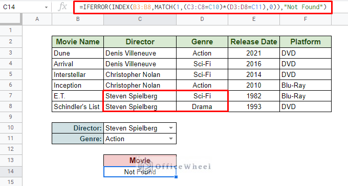
For an in-depth breakdown of this method, please have a look at our Use of Google Sheets INDEX MATCH in Multiple Columns article.
2. Using VLOOKUP to Match from Multiple Columns
Next up we have the traditional way to lookup values through matches in Google Sheets, and that is by using the VLOOKUP function.
However, compared to INDEX-MATCH, VLOOKUP has some technical limitations:
The function only looks towards the right. VLOOKUP can only extract values with a column index. Since column indexes start from 1 and move to the right, the function does the same.
Needs a special column for multiple columns or criteria. The function has no field for multiple criteria, thus you have to create a separate column (anywhere to the left of the column that is to be extracted).
It is always better to see through an example, and we will go over the process step-by-step.
For our example, we will try to extract the Release Date of a movie based on its name and genre as the two match criteria.
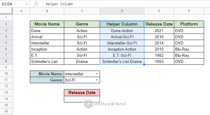
Step 1: Create a “Helper Column” to concatenate the multiple column values into one. You can use any form of delimiter as long as it matches our search key field in our formula. We have used a hyphen (-) delimiter.
It is very important to make sure that the helper column is on the left of the column whose values we are going to extract.
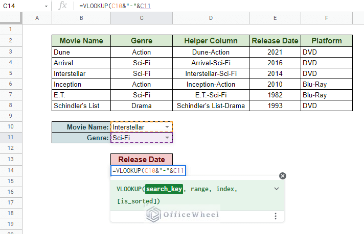
Step 2: Open the VLOOKUP function at the target and enter the search key. Our search key is the combination of the two criteria that are located in cell C10 and C11 respectively. Make sure the search key matches the format of the helper column.
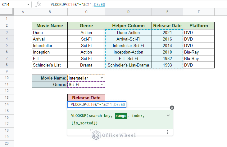
Step 3: Input the range. For us, this includes the Helper Column and Release Date columns.
Step 4: Since the values we are looking to extract are in the Release Date column, the selected range places it in index 2.
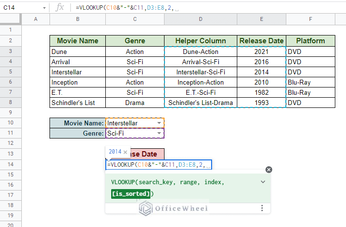
Step 5: We will leave the [is_sorted] field as FALSE. Close parentheses and press ENTER.
Our final formula:
=VLOOKUP(C10&"-"&C11,D3:E8,2,FALSE)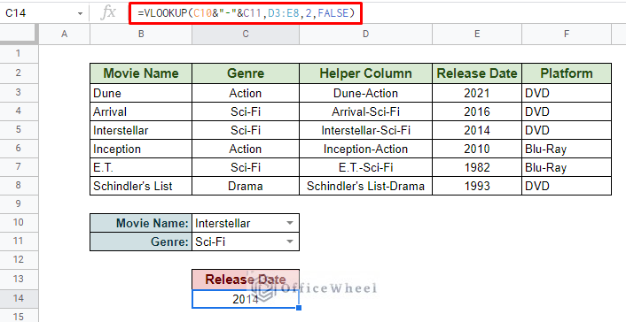
Read More: Alternative to Use VLOOKUP Function in Google Sheets
Special Case: Match from Different Sets of Data in Google Sheets
In the following worksheet, we have two sets of data for Dorm 1 and Dorm 2. Each of these dorms has its residents’ names and their countries of origin.
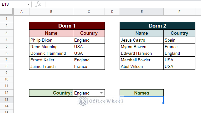
For our task, we will try to extract the Names by matching them with the asked Country of origin that is in cell C12.
The data to be extracted are in two separate columns and so are our match data. This means that we are unable to use the traditional approaches that we have just discussed in our previous two methods.
For this reason, we will take advantage of the array formula, FILTER, and we will couple it up with the MATCH function.
Our formula:
=FILTER({B4:B8;E4:E8},MATCH({C4:C8;F4:F8},C12))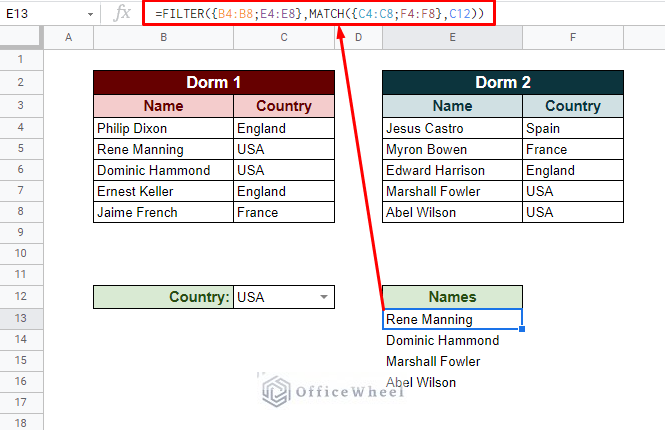
Note: This is a special case and may not work for all situations.
Final Words
That concludes all the ways you can use to match from multiple columns in Google Sheets. We hope that the methods will come in handy for your spreadsheet tasks.
Feel free to leave any queries or advice you might have for us in the comments section below.
Related Articles
- [Fixed!] INDEX MATCH Is Not Working in Google Sheets (5 Fixes)
- Use INDEX MATCH Across Multiple Sheets in Google Sheets
- Combine VLOOKUP and HLOOKUP Functions in Google Sheets
- Google Sheets HLOOKUP to Return Column (3 Simple Ways)
- Match Multiple Values in Google Sheets (An Easy Guide)
- How to Create Dependent Drop Down List in Google Sheets
- INDEX-MATCH with Multiple Criteria in Google Sheets (Easy Guide)
- Find Cell Reference in Google Sheets (2 Ways)