Lock Cell Reference in Google Sheets (3 Ways)

One of the problems that many bookkeepers, financiers, or anyone who works with worksheets will have in common is the understanding and the application of locking cell references.

So now with Google Sheets on the constant rise, we will take this opportunity to help you understand how to lock cell references in Google Sheets worksheets.

But first, let us clarify your understanding of regular cell references and why we need to lock them in place for certain situations.

Table of Contents

Relative vs. Absolute: Why Do We Need to Lock Cell Reference in Google Sheets?

Relative cell references are the most common way we refer to cells in a worksheet.

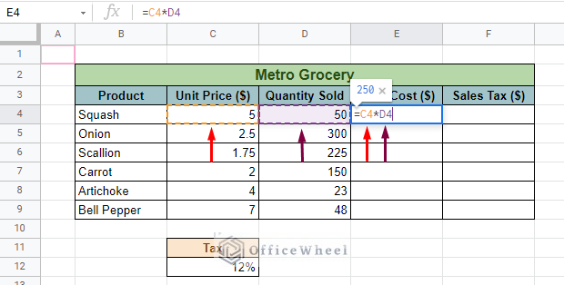
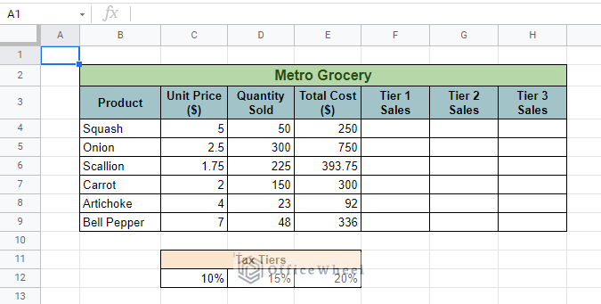
For example, in the following worksheet, we are first going to calculate the total cost of our first product, Squash.

We will be doing this in cell E4, and thus our formula will be

=C4*D4

Here, C4 and D4 are our cell references.

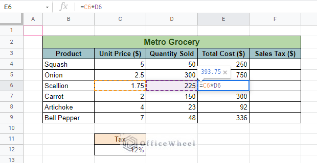
Now, if we drag the formula down the column using the fill handle, we will notice that at every new row the cell reference is changing. They are changing relative to the new row, and thus we call them Relative Cell References.

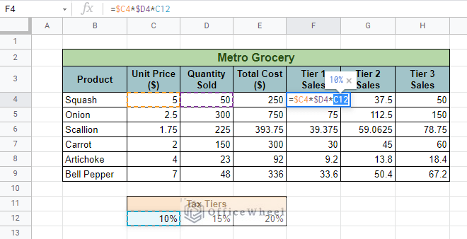
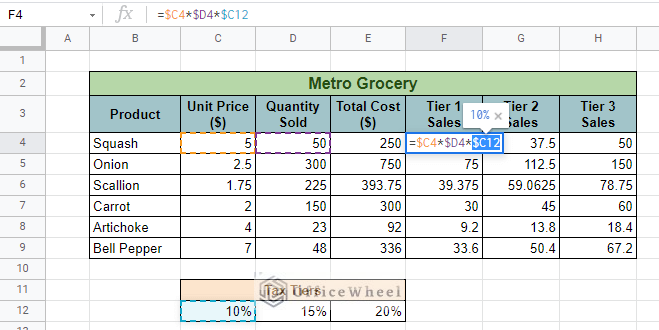
Now let’s try the same with the Sales Tax column. Here, our formula will be:

=C4*D4*C12

Where cell C12 contains our Tax rate.

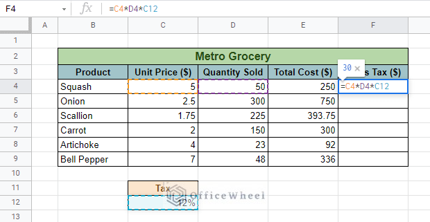
What happens if we apply this formula the same way we did just before with the fill handle?

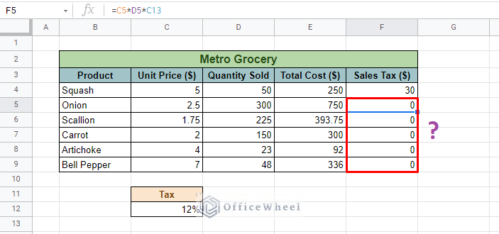
Our table is giving the wrong answers for the rest of the column. This is because for every new row the reference cells are changing for the Tax rate cell as well. Notice the formula bar on the previous image, where the Tax cell reference should have been C12, it has moved to C13.

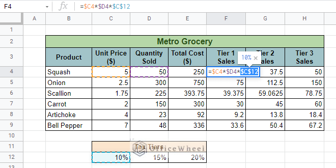
So, for this Tax cell in particular, we have to lock the reference down. We do this by adding a dollar sign ($) in front of the column and row numbers. Our formula at cell F4 becomes:

=C4*D4*$C$12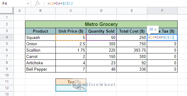

Now let’s apply this to the rest of the column.

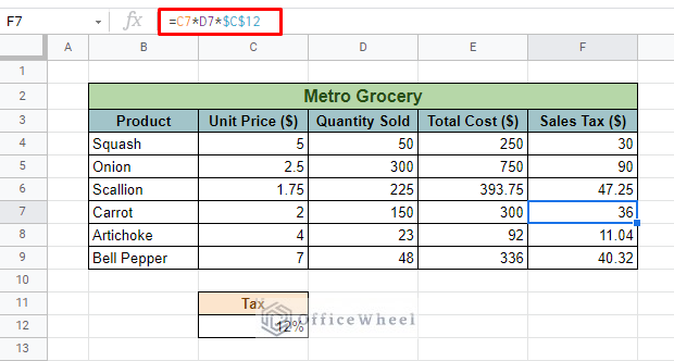
As you can see that the Tax cell, cell C12, is locked in place for all of the rows in this column.

We call this locked form Absolute Cell Reference. And they are of three types:

Name	Example	What it does
Absolute Cell Reference	$C$12	Locks both column and row numbers
Mixed Cell Reference (Column)	$C12	Locks only the column number
Mixed Cell Reference (Row)	C$12	Locks only the row number

3 Ways to Lock Cell Reference in Google Sheets

1. Absolute Cell Reference

Having understood the importance of having locked cells, let us now dive into the most used type of Absolute Cell Reference.

So, if I choose to lock down cell C12, I will be adding the dollar sign ($) in front of both C (column number) and 12 (row number). The locked cell will look like: $C$12.

We have already discussed in detail the differences between relative and absolute cell references in the previous section. To recap, let’s see the following set of images.

Our dataset and its formulas in their respective cells.

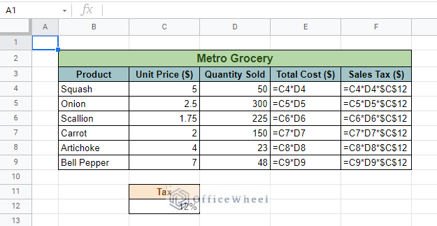
Note: To view the formulas of each cell in the worksheet, navigate to the View tab > Show > Formulas. Or just use the keyboard shortcut: CTRL + `

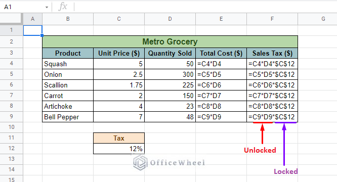
No matter where we copy this formula to, the cells locked by the absolute ($) will not change.

2. Mixed Cell Reference (Lock Column)

To put it quite simply, Mixed Cell Reference is just another form of Absolute Cell Reference. This is because they focus on either locking the columns or the rows part of the cell reference.

As you may have already understood, situations, where you have to lock either column or row, can be rare beyond very sophisticated formulas.

Either way, let’s first look at the column version of mixed cell references.

As you can see, we have brought some changes to our dataset:

We have added Tax Tiers to our data. Calculating the new Sales Tax for each tier is easy, but having the correct formula in each cell requires us to be a bit more creative.

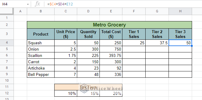
In column Tier 1 Sales we have to lock in columns C and D. If we don’t, this happens when we use the fill handle to cover the tiers of Sales Tax (fill handle to the right):

As you can see, only the Tax Tier cell, cell D12, is correctly implemented, but the other two references are wrong. This is understandable because, as we dragged the fill handle to the right, the references have also moved to the right.

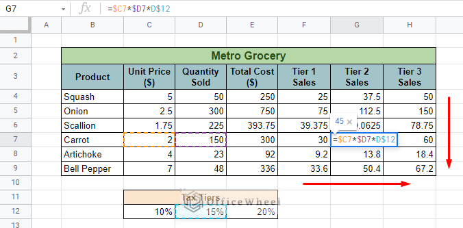
To rectify this issue, we must lock columns C and D only so that Google Sheet’s natural reference selection does not move to the right while keeping the correct reference as we move down the column. We do this by adding the absolute ($) before C and D in cell F4.

=$C4*$D4*C12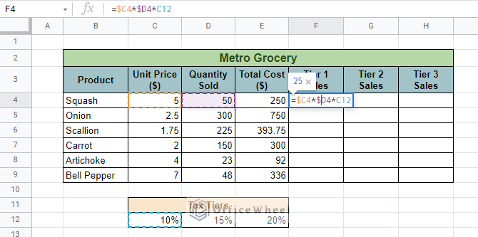

The new result after using fill handle horizontally:

Great! We have successfully locked the columns of our formula. Now, no matter how far we move with the fill handle, the column references will remain static.

Similar Readings

3. Mixed Cell Reference (Lock Row)

Let us now see what happens when we use the fill handle from cell F4 down the column this time.

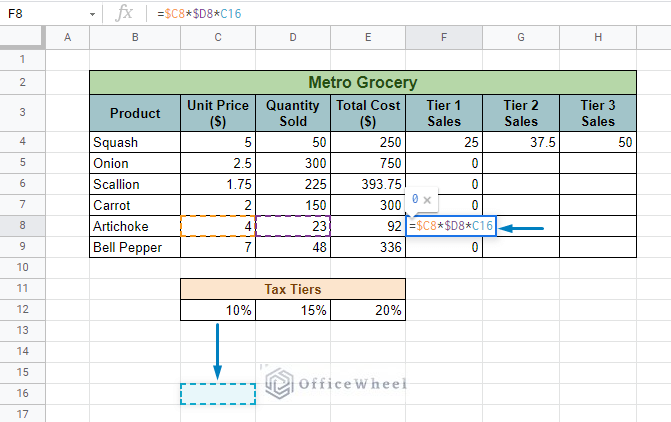
This is the same problem that we faced before we applied Absolute Cell Reference in our first dataset. As we pulled down the fill handle, Google Sheets has also naturally referred to lower cells from the initial point.

We must apply a lock to the Tax cells. But absolute cell reference will not work here the same way it did in method 1. This is because the absolute cell reference ($C$12) will lock on to cell C12 only. We have to allow the cells to refer to cells D12 and E12 as well.

To work around this restriction, we will only be putting the absolute ($) before the row number, in this case, 12.

So now the formula at F4 becomes:

=$C4*$D4*C$12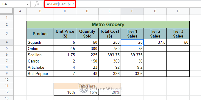

With our formula reaching its final form, let’s fill the rest of the cells in our table.

And done! We have successfully applied mixed cell references to our new dataset.

Keyboard Shortcut: The F4 Cycle

What if we told you that you can cycle through the three types of Absolute Cell References with just a click of a button?

Well, it is possible thanks to the F4 key shortcut.

Simply highlight the cell reference that you want to lock:

Press the F4 key once for Absolute Cell Reference:

Press the F4 key twice for Mixed Cell Reference (Lock Row)

Press the F4 key a third time for Mixed Cell Reference (Lock Column)

Press the F4 key one final time to go back to the unlocked cell:

We like to call the F4 Shortcut Cycle.

You may already know, but the F4 key is quite the versatile shortcut for Google Sheets.

Final Words

Understanding and applying locks to your cell references are integral to your worksheet experience, whether you are using Google Sheets or any other worksheet application. At least for Google Sheets, we hope that this article helped you understand absolute cell reference and its iterations better.

If you feel like we have missed anything, or if anything is unclear, please feel free to drop a comment.