Google Sheets: Conditional Formatting Row Based on Cell

Conditional formatting is quite a versatile function in any spreadsheet application. And today we will see the conditional formatting of a row/rows based on a cell in Google Sheets.

Basics of Conditional Formatting a Row in Google Sheets

We start by understanding some key points and steps involved when conditionally formatting a row in Google Sheets.

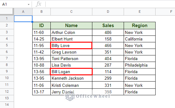
Here we have a typical dataset of different values which will allow us to check for different types of conditions:

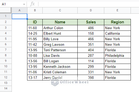
For our example, we will highlight all the rows that contain the region, Florida.

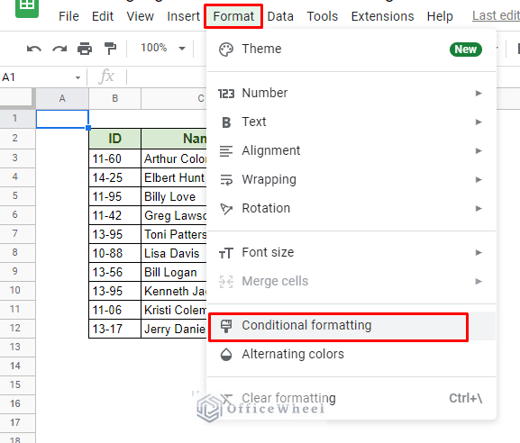
Step 1: Navigate to Conditional Formatting from the Format tab.

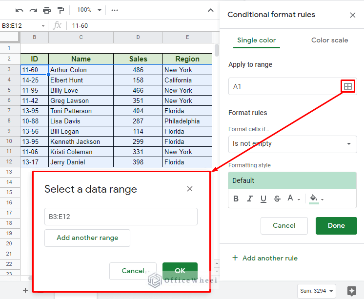
Step 2: The first thing we do in the Conditional format rules menu is to determine our formatting range (if you haven’t already done it). Click on the grid icon in the Apply to range section to open the Select a data range window. Simply input or select the range of cells from your worksheet. Click OK  to apply.

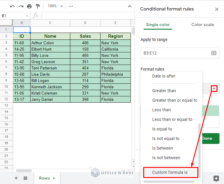
Step 3: Next is the most important part of our process, the formatting rules, namely the formulas we are going to apply. To inout our  custom formulas in conditional formatting, click the drop-down menu under the Format cells if… section to find the Custom formula is option at the bottom of the list.

Step 4: Our highlight condition was: Highlight all rows from the Florida Region. So, our formula will be:

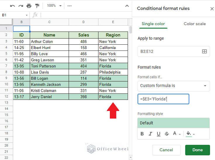
The absolute ($) added in front of the column E reference means that the column is fixed whereas the row references are free to move, thus the formatting is painted across the entire row.

Step 5: Choose the type of formatting you want to apply and click Done to finish.

To learn more about conditional formatting rows according to different types of cell values, please visit our Change Row Color Based on Cell Value in Google Sheets article.

With the basics out of the way, let’s see some scenarios where conditional formatting based on cell comes in handy.

Read More: Conditional Formatting with Multiple Conditions Using Custom Formulas in Google Sheets

Other Scenarios of Conditional Formatting Row Based on Cell in Google Sheets

1. Conditional Formatting Row With a Value Based on a Different Cell

Continuing from our last example, we will once again try to highlight rows according to region, but this time, our Region name will come from another cell in the worksheet.

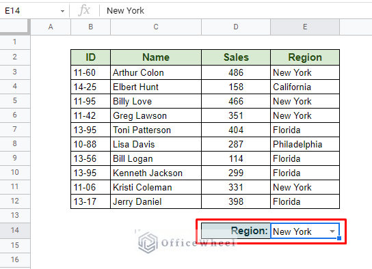
The drop-down list, located in cell E14, contains all the region names of our dataset. We will be using this cell as a reference in our custom formula.

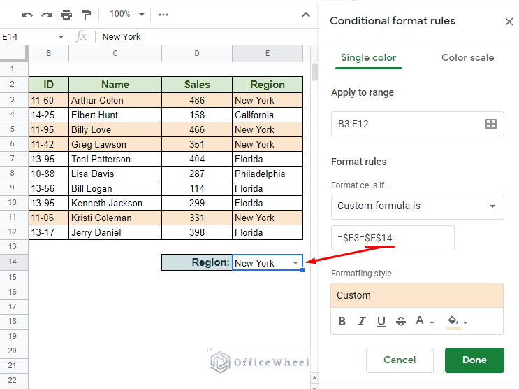
Note: You must apply absolute cell reference to the condition cell (cell E14 in our case, $E$14) otherwise the rows will not be highlighted properly.

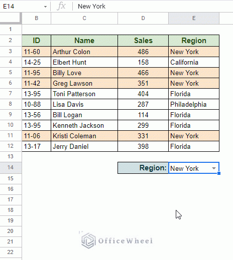
Our custom formula in action:

Please visit our Conditional Formatting Based on Another Cell in Google Sheets to learn more and see more examples.

Read More: Highlight Row If Cell Contains Text with Conditional Formatting in Google Sheets

2. Using Regular Expressions

We can already see the use of custom formulas in conditional formatting in Google Sheets. We can take it a step further with these formulas to lookup certain strings within the selected range and highlight the row matches.

For example, we could look up partial text matches, like the name “Bill” from the dataset.

However, with a general formula, this won’t be possible since Google Sheets cannot recognize partial text. For that, we have to use Regular Expressions, and by extension, the REGEXMATCH formula.

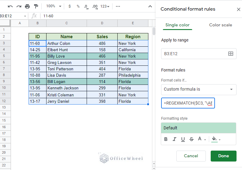
Read More: Use REGEXMATCH Function for Multiple Criteria in Google Sheets

Similar Readings

• How to Use Nested IF Function in Google Sheets (4 Helpful Ways)
• Use IF and OR Formula in Google Sheets (2 Examples)
• How to Use VLOOKUP for Conditional Formatting in Google Sheets
• Use Multiple IF Statements in Google Sheets (5 Examples)

3. Based on Checkboxes

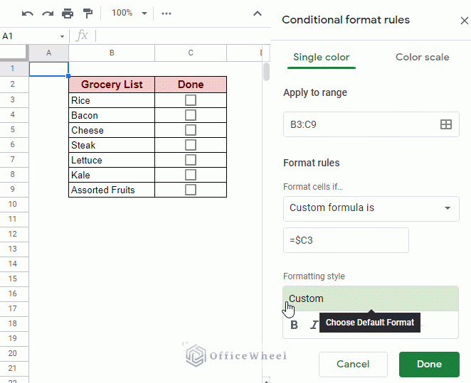
Let’s move to something much simpler in our next example. Data validation techniques like checkboxes are widely used in many spreadsheets.

What if we want to go a step further and use conditional formatting to highlight the rows that have been checked?

The custom formula for it is quite simple:

Since C3 contains our condition and we are checking if the condition is TRUE or FALSE. If TRUE, the conditional formatting will highlight the row.

Read More: Conditional Formatting with Checkbox in Google Sheets

4. Based on Multiple conditions

In our final example, we will try to highlight an entire row based on multiple conditions. We already know that conditional formatting in Google Sheets works in Boolean, meaning if the condition stated by the user is TRUE, we get a highlighted cell.

Understanding that, for multiple conditions, we can approach our custom formula by making sure that all conditions are TRUE (AND format) or if just one condition is TRUE (OR format)

Luckily, we have AND and OR functions in Google Sheets to help us with that.

For now, let’s highlight rows for the following conditions:

1. Region: New York
2. Sales: More than 400 units

Since we want both conditions to be TRUE, we will use the AND function. Thus, our formula to highlight the rows satisfying these conditions will be:

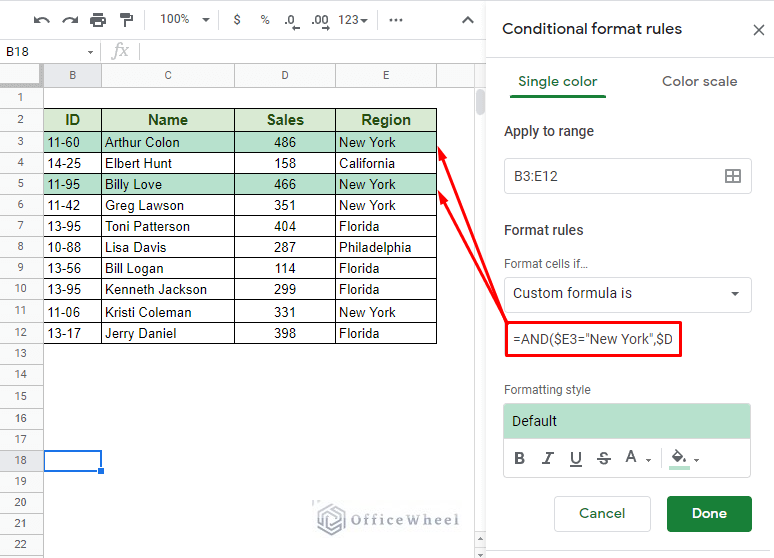
Again, to highlight the entire row, our cell reference needs only to have the column references locked with absolutes ($).

Read More: Google Sheets: Conditional Formatting with Multiple Conditions

Final Words

That should cover how we can conditionally format a row based on cell in Google Sheets with some extra examples to clarify its potential. We hope that the discussion of the various scenarios comes in handy for your tasks.

Feel free to leave any queries or advice you might have for us in the comments section below.

Related Articles

• Highlight Duplicates in Google Sheets (4 Ways)
• How to Do IF THEN in Google Sheets (3 Ideal Examples)
• Search in All Sheets in Google Sheets (An Easy Guide)
• How to Use IF Function in Google Sheets (6 Suitable Examples)
• Highlight Duplicates in Two Columns in Google Sheets (2 Ways)
• Pivot Table Formatting in Google Sheets (3 Easy Ways)
• Copy Formatting From One Sheet To Another In Google Sheets (2 Ways)