We are aware of using single IF statements in Google Sheets for getting values logically. But we don’t know much about how to use multiple IF statements in Google Sheets. It is a bit tricky. In this article, I’ll show 5 useful examples to use multiple IF statements in Google Sheets with clear images and steps.
A Sample of Practice Spreadsheet
You can download Google Sheets from here and practice very quickly.
5 Suitable Examples to Use Multiple IF Statements in Google Sheets
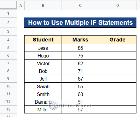
Let’s get introduced to our dataset first. Here we have some students in Column B and their marks in Column C. Now we want to put their grades in Column D. The grading system would be like this:
| Grade | Criteria |
|---|---|
| A | Marks > 80 |
| B | Marks < 80 |
| C | Marks < 70 |
| D | Marks < 60 |
So I’ll show 5 suitable examples to use multiple IF statements in Google Sheets with the help of the dataset given below.
Example 1: Combining Multiple IF Functions
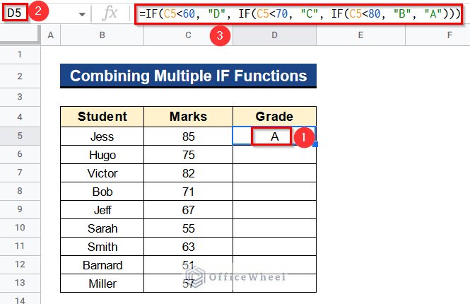
We can combine multiple IF functions to use multiple IF statements in Google Sheets. Combining the multiple IF functions will give our desired grade instantly.
Steps:
- Firstly, type the following formula in Cell D5–
=IF(C5<60,"D",IF(C5<70,"C",IF(C5<80,"B", "A")))- Secondly, hit Enter to get the desired grade.
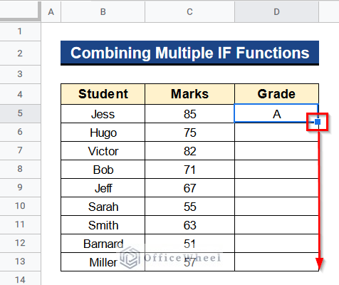
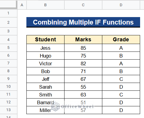
- Finally, you’ll get your desired result like below.
Read More: Google Sheets IF Statement in Conditional Formatting
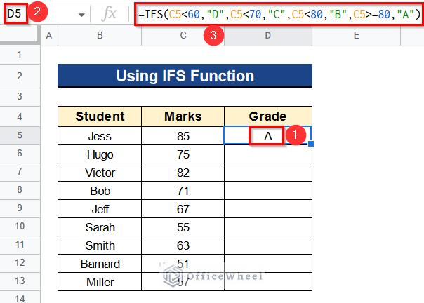
Example 2: Using IFS Function
In addition to our previous examples, we can simply use the IFS function in Google Sheets. This function single-handedly gives the result we previously got by using multiple IF functions together. We don’t have to use the IF function again and again if we use the IFS function.
Steps:
- First, write the following formula in Cell D5–
=IFS(C5<60,"D",C5<70,"C",C5<80,"B",C5>=80,"A")- Second, press Enter to get the desired result.
- Then, use the Fill Handle tool to get the results in the rest of the cells.
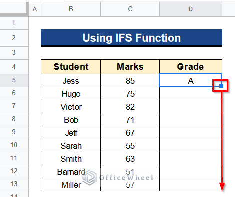
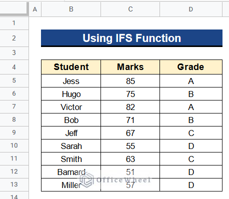
- At last, you’ll get something like this.
Read More: How to Do IF THEN in Google Sheets (3 Ideal Examples)
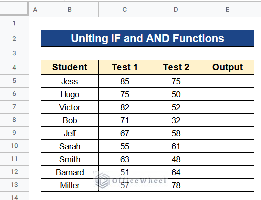
Example 3: Uniting IF and AND Functions
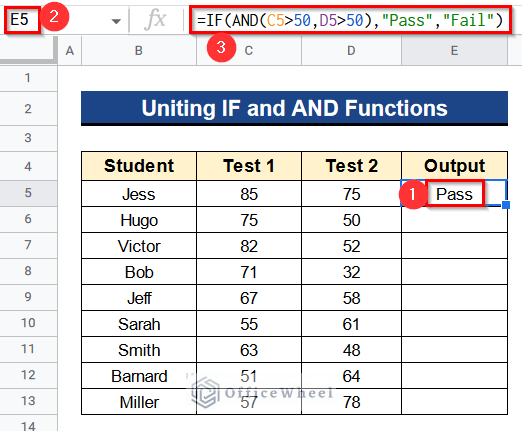
Now we have a different dataset like below. We have some students in Column B, their test 1 scores in Column C, and their test 2 scores in Column D. We want our output as Pass or Fail based on the criteria. The criteria are that any student has to get over 50 marks in both tests to get Pass. Otherwise, he’ll get Fail. So we can do this procedure by uniting the IF and AND functions together. The result will be instant.
Steps:
- First of all, insert the following formula in Cell E5–
=IF(AND(C5>50,D5>50),"Pass","Fail")- Next, click Enter to get the output.
Formula Breakdown
- AND(C5>50,D5>50)
First of all, this function will return TRUE if the values of Cell C5 and D5 both are greater than 50 otherwise FALSE.
- IF(AND(C5>50,D5>50),”Pass”,”Fail”)
Consequently, this function then gives the output as Pass if the criteria are TRUE otherwise it gives Fail.
- After that, apply the Fill Handle tool like below to get all the results.
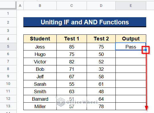
- At last, you’ll see that there is either Pass or Fail in all the cells of Column E.
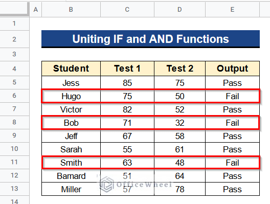
- Moreover, you may notice that only 3 students from Row 6,8, and 11 get a Fail because they can’t get over 50 marks on both tests.
Read More: Filter Values that Contains Multiple Text Criteria in Google Sheets (2 Easy Ways)
Similar Readings
- Use REGEXMATCH Function for Multiple Criteria in Google Sheets
- How to Use VLOOKUP for Conditional Formatting in Google Sheets
- Find if Date is Between Dates in Google Sheets (An Easy Guide)
- How to Use ARRAYFORMULA with IF Function in Google Sheets
Example 4: Merging IF and OR Functions
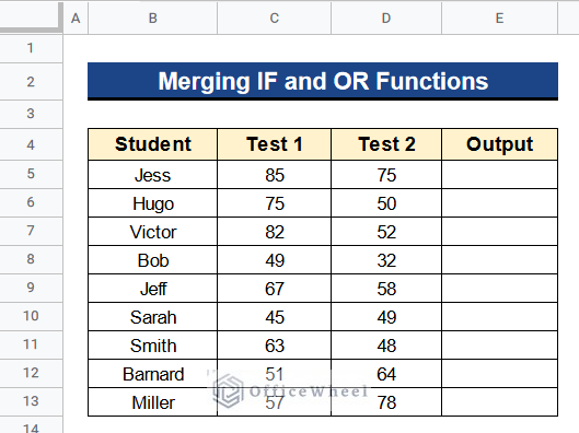
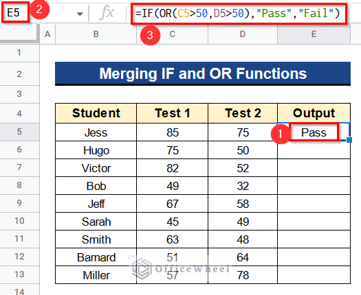
At this moment, we have a dataset below similar to the former example. But now we’ll set different criteria. Now any student will get a Pass if he only gets over 50 marks in any of the 2 tests. We’ll do this by merging the IF and OR functions. Let’s see how to do it.
Steps:
- In the first place, type the next formula in Cell E5–
=IF(OR(C5>50,D5>50),"Pass","Fail")- Afterward, hit the Enter Button to get the output as Pass or Fail.
Formula Breakdown
- OR(C5>50,D5>50)
Firstly this function will return TRUE if any value from Cell C5 or D5 is greater than 50 otherwise FALSE.
- IF(OR(C5>50,D5>50),”Pass”,”Fail”)
Finally, this function gives the output as Pass if the criteria are TRUE. If the criteria are FALSE then it gives Fail.
- Again, use the Fill Handle tool to get the rest of the results.
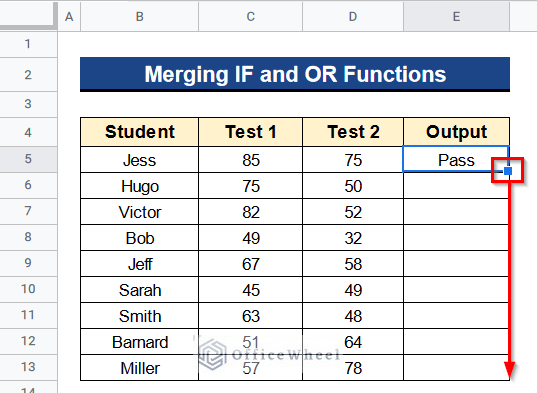
- Ultimately, we’ll get our desired output in Column E.
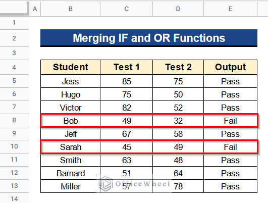
- You’ll find out that only 2 students of Row 8 and 10 got a Fail because they can’t fulfill the criteria. They got less than 50 marks on both tests.
Read More: How to Use IF and OR Formula in Google Sheets (2 Examples)
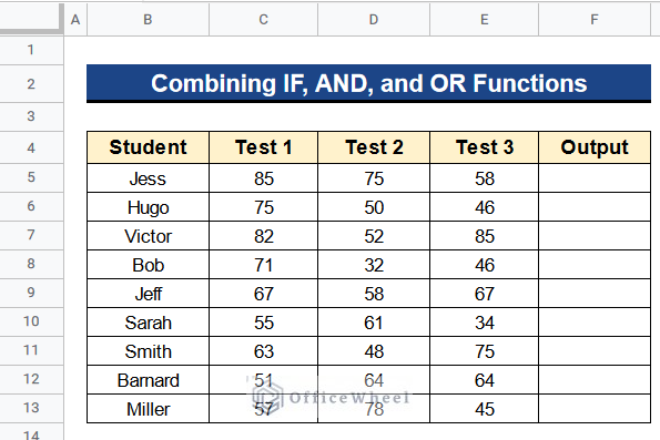
Example 5: Combining IF, AND, and OR Functions
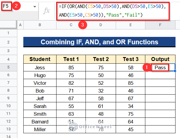
We have extended our dataset for setting new criteria. Now we have 3 test numbers. We want that any student will get a Pass if he gets over 50 marks in any 2 of the 3 tests. Otherwise, he will get a Fail. For this purpose, I’ll combine the IF, AND, and OR functions to get our desired output.
Steps:
- Before all, write the next formula in Cell F5–
=IF(OR(AND(C5>50,D5>50),AND(D5>50,E5>50), AND(E5>50,C5>50)),"Pass","Fail")- Then, press the Enter Button to get the result.
Formula Breakdown
- AND(C5>50,D5>50)
Earlier on this function returns TRUE if both values from Cell C5 and D5 are greater than 50 otherwise FALSE.
- AND(D5>50,E5>50)
This also works like the previous one. But it works for Cell D5 and E5.
- AND(E5>50,C5>50)
This is also the same but works for Cell E5 and C5.
- OR(AND(C5>50,D5>50),AND(D5>50,E5>50), AND(E5>50,C5>50))
Next, this OR function gives TRUE if any one of the 3 AND functions matches the criteria. Or it will give FALSE.
- IF(OR(AND(C5>50,D5>50),AND(D5>50,E5>50), AND(E5>50,C5>50)),”Pass”,”Fail”)
At last, this IF function gives the output as Pass if all the criteria are TRUE otherwise the output will be Fail.
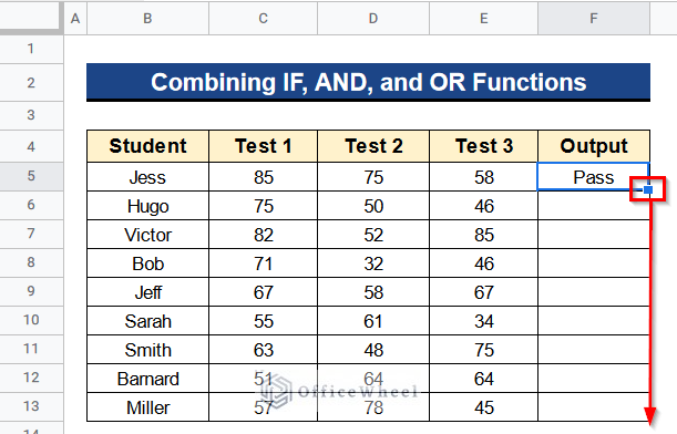
- Moreover, assign the Fill Handle tool in order to get results in all the cells of Column F.
- In the end, we’ll get our desired output as Pass or Fail in Column F.
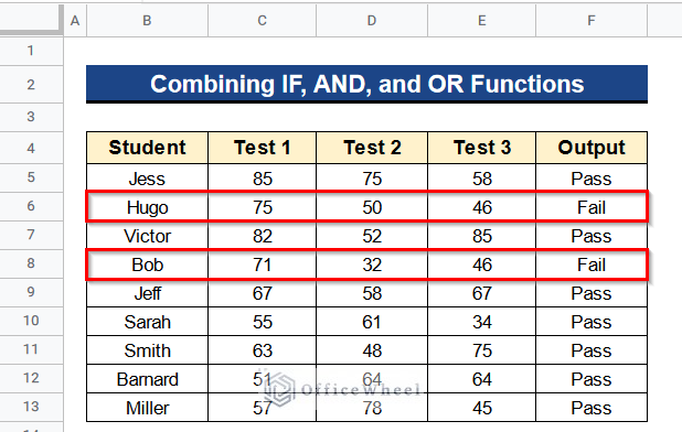
- Only 2 students of Row 6 and 8 got a Fail because they can’t get over 50 marks in any 2 tests out of the 3 tests.
Read More: Conditional Formatting with Multiple Conditions Using Custom Formulas in Google Sheets
Conclusion
That’s all for now. Thank you for reading this article. In this article, I have discussed how to use multiple IF statements in Google Sheets. I have shown 5 suitable examples for this purpose. Please comment in the comment section if you have any queries about this article. You will also find different articles related to google sheets on our officewheel.com. Visit the site and explore more.
Related Articles
- How to Use Nested IF Statements in Google Sheets (3 Examples)
- Highlight Cell If Value Exists in Another Column in Google Sheets
- Use Nested IF Function in Google Sheets (4 Helpful Ways)
- If Cell Contains Text Then Return Value in Another Cell in Google Sheets
- How to Use IF Condition Between Two Numbers in Google Sheets
- Match Multiple Values in Google Sheets (An Easy Guide)