Any type of formatting based on cell values or conditions can be easily done by the Conditional Formatting option of Google Sheets.
To show you how to change row color based on cell value in Google Sheets, we will be using the following dataset:
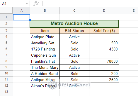
Each column has unique sets of values that we will be using as various conditions to conditionally format our table.
Let’s get started.
4 Ways to Change Row Color Based on Cell Value in Google Sheets
1. Change Row Color Based on Text Value
For our first condition, we will be looking at text values in cells.
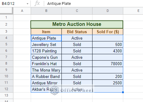
Step 1: Highlight data range. Select all the cells over which you want to apply conditional formatting on.
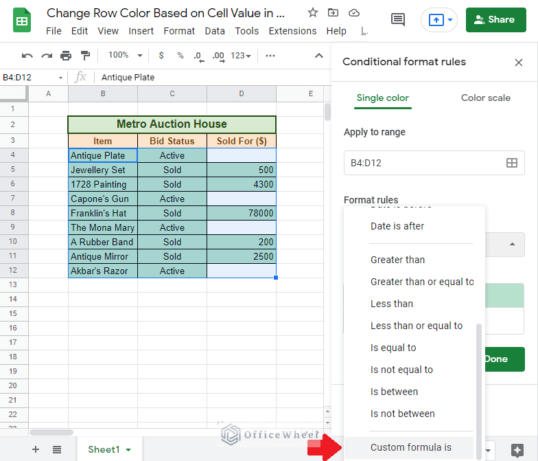
Step 2: From the top menu ribbon, select Format tab > Conditional Formatting.
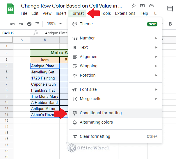
This will open the Conditional formatting rules menu tray on the right side of the window, with some default formatting already applied.
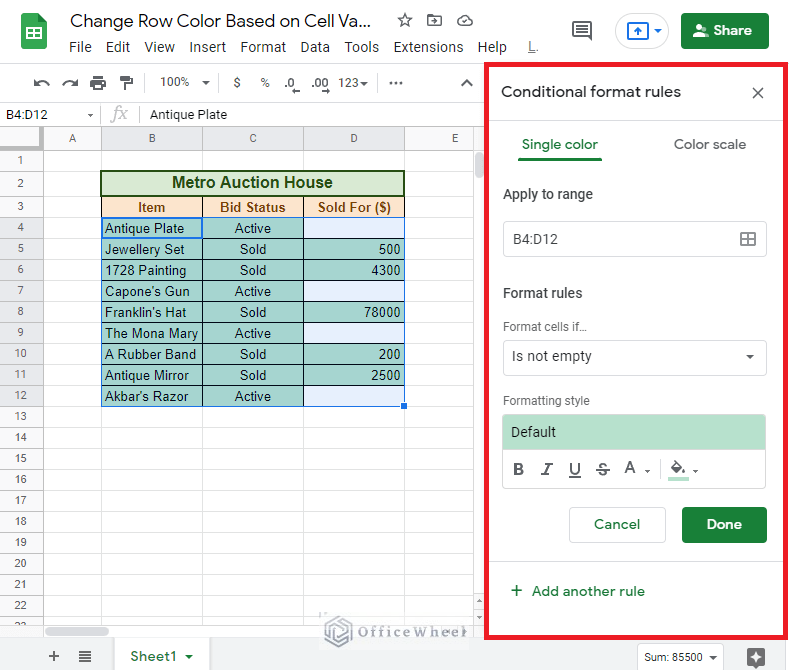
Step 3: Click on the drop-down menu under Format cells if… and scroll to the bottom to find the Custom formula is option. A custom formula is necessary if we want to specifically highlight entire rows within our selection.
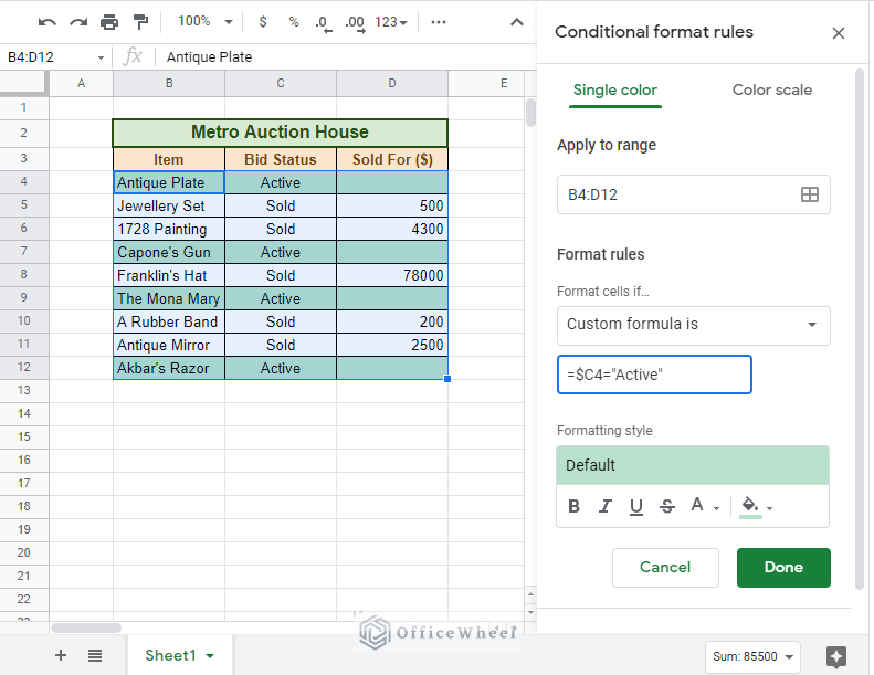
Here we enter the formula =$C4=”Active” as our custom formula.
Formula Breakdown:
- $C4: Our starting cell in our selection. The absolute sign ($) will help lock the column reference in place as we move down the row, which remains unlocked. (More on Locking Cell Reference: Link)
- =”Active”: It is the condition we are checking for. We could also have given “Sold” as the other condition for this column.
Step 4: You can customize your conditional highlights from the Formatting style section.
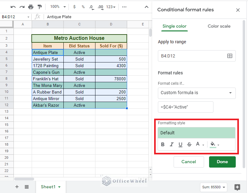
Step 5: Click Done once you are satisfied with your conditional formatting.
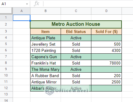
As you can see, we have successfully changed the row colors of the entire row that contained the value “Active” from the Bid Status column.
2. Change Row Color Based on Numerical Conditions
Now, let’s move on to some numerical conditions for our highlights. To show this, we will be applying the condition that highlights rows that have a Sold For value greater than $3000.
We start off the same way.
Step 1: Open the Conditional formatting rules menu tray. Format tab > Conditional Formatting.
Step 2: Choose the custom formula option. Format cells if… > Custom formula is.
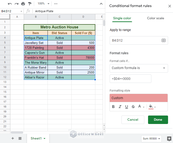
Step 3: Apply the custom formula. In our case, it is =$D4>3000.
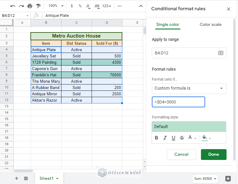
Formula Breakdown:
- $D4: Our starting cell in our selection. The absolute sign ($) will help lock the column reference in place as we move down the row, which remains unlocked.
- >3000: It is the condition we are checking for. We will highlight all the rows that have a value greater than 3000 in the Sold For column.
Step 4: Add some more formatting from the Formatting style section.
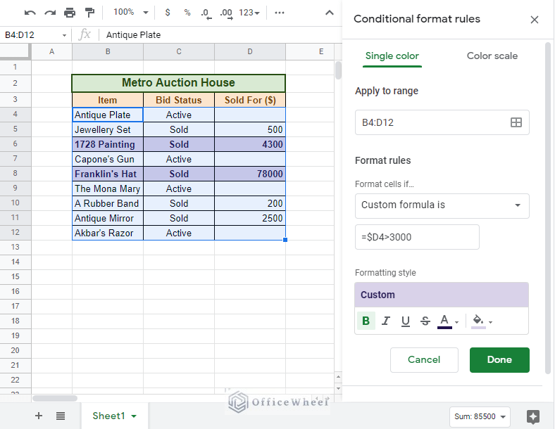
Step 5: Click Done.
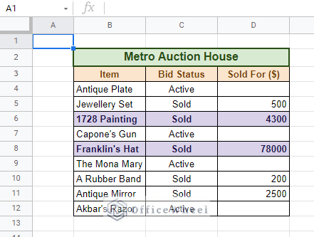
The rows that contain values greater than $3000 in the Sold For column have been successfully formatted.
3. Using Advanced Custom Formula to Change Row Color
Conditional formatting in Google Sheets does not restrict us to simple formulas as we have seen in the previous methods. If you are good enough to know your way around the various functions of Google Sheets, then you will have no problems handlings some unique formulas that can be used with conditional formatting.
Let’s have a look at a couple of these examples:
I. Find Specific String (VLOOKUP)
In this example, we aren’t really going to be using the VLOOKUP function, but we will be doing something similar to it in Conditional Formatting.
We aim to highlight all the rows that have the bidding status “Sold”.
But instead of writing the condition within the formula, we will be extracting/comparing it to another cell within the worksheet.
We shall be using a combination of the MATCH and INDIRECT functions to mimic VLOOKUP:
=match($C4,indirect("Sheet1!F3"),0)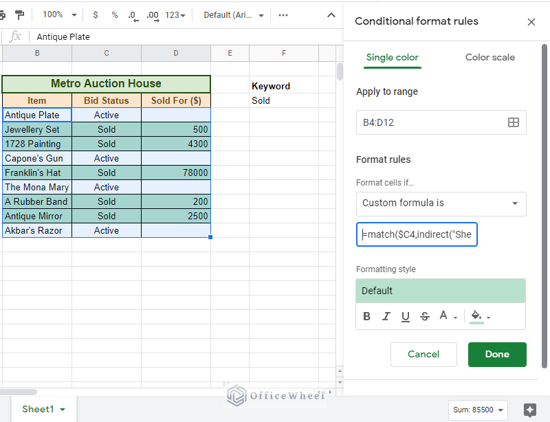
The advantage of using this formula, over that of method 1, is that we can add multiple conditions to it. In other words, as long as we have necessary conditions written down in a single column (Keyword column, column F in our case), we can highlight all the given conditions if we just change our range of accepted values from $F3 to $F3:F.
II. Highlight Rows with Specific Name/Word
In the next example, we will be using the unique Regular Expression function of Google Sheets, REGEXMATCH.
We will be using this function to highlight rows that have the word “Antique” in them, in the Item column. This is essentially looking for a partial match.
The formula is:
=REGEXMATCH($B4, "\AAntique\s*([^\n\r]*)")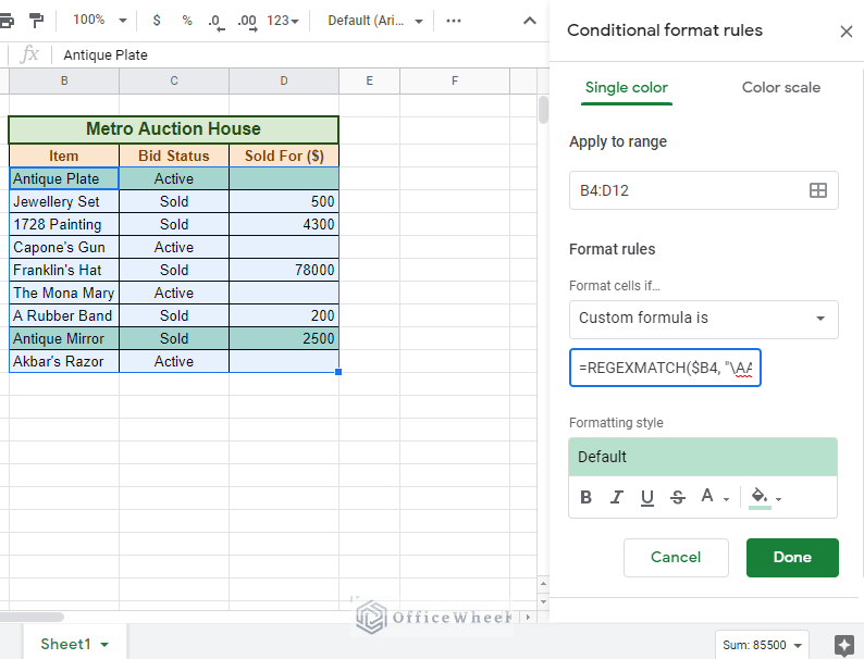
The advantage of using this formula is that, no matter how long the string is in the respective cell, the formula will only check the input string specifically. It doesn’t matter if the desired length of the string is in the beginning, middle, or end of the text.
These are some advanced examples that we have just discussed. You are free to utilize them if your workbook caters to these specific conditions. All you have to do is change the conditions and the range for your spreadsheet.
4. Applying Multiple Rules to Change Row Color
With enough ingenuity, you can apply multiple conditions to a single Conditional Format in Google Sheets. However, you can’t apply two different Conditional Formats at once. But as a workaround, Google Sheets does provide us with its Conditional format rules menu tray to add, edit, and track all of the conditional formats in the worksheet.
To show this we will be continuing from method 1 and add method 2 from this Conditional format rules menu tray.
Step 1: Open the Conditional formatting rules menu tray. Format tab > Conditional Formatting.
Step 2: If your worksheet already has a conditional format applied to it then your tray will look like this:
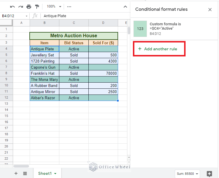
Click on Add another rule to add the second format to this sheet.
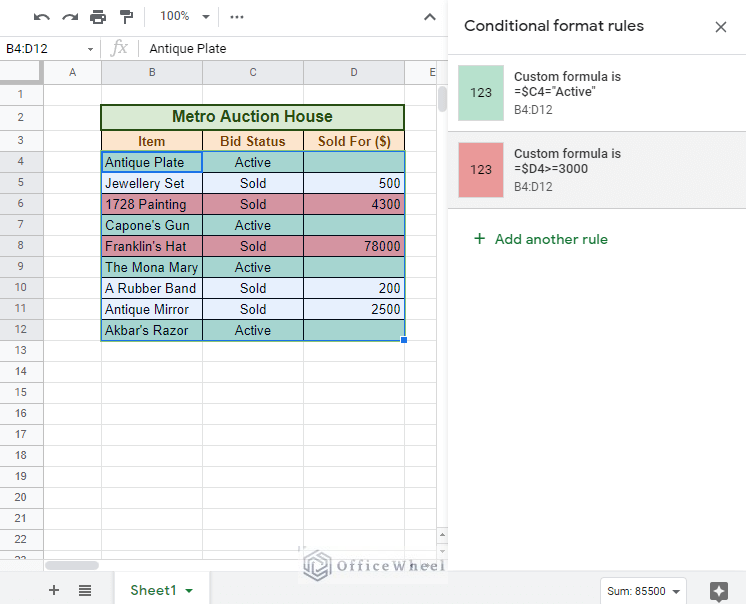
Step 3: Let’s add the same formula that we applied in method 2.
Step 4: Click Done. You will see both conditions highlighted in your worksheet and both of the conditional formats on the menu tray.
Final Words
Changing row colors in Google Sheets according to cell values is so much easier with conditional formatting. We have tried to give you all the iterations of how to achieve it in this article, and we hope you can apply them to your worksheets promptly.
If you have any questions or suggestions, feel free to comment.