Google Sheets has many formulas that make working considerably simpler. The IF THEN logical calculation in Google Sheets is one of the amazing features that make it easy to verify logical arguments, single or multiple criteria, or conditions, and return a value if they are TRUE or a different value if they are FALSE.
A Sample of Practice Spreadsheet
You can copy the spreadsheet that we’ve used to prepare this article.
3 Ideal Examples to Do IF THEN in Google Sheets
We can use the IF function by itself in a single logical test or nest numerous IF statements into one formula to create more complicated tests.
The IF Function has the following syntax:
=IF(logical_test, value_if_true, value_if_false)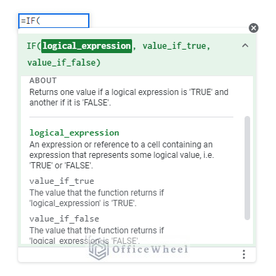
There are multiple methods to use the IF statement followed by a THEN outcome in Google Sheets. In Google Sheets, we may combine several IF statements to run a longer and more complex logical test. To improvise calculations and logical tests, we can nest some other functions as well.
1. Utilizing IF THEN with Single Condition
Use the IF function in your Google Sheets formula if you want to conduct a logical test that returns different answers depending on whether the test is TRUE or FALSE. Use it in Google Sheets by following these steps.
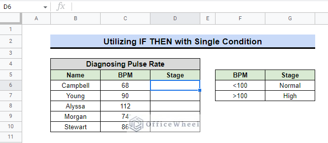
Assume we have a dataset with a few patients’ most current pulse rates. We must ascertain the state of the patient’s blood pressure. If the rate exceeds 100, then the patient has excessive or high blood pressure.
Steps:
- We will choose cell D6 initially.
- First and foremost, we’ll use the following formula as the first logical argument:
=IF(C6<100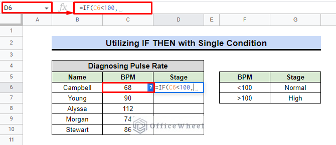
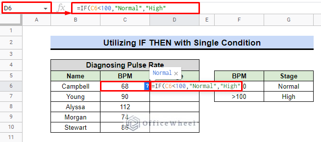
- After that, we’ll apply the following formula:
=IF(C6<100,"Normal","High"- The value to return in this case if the logical argument is TRUE is “Normal”.
- If the logical argument is FALSE, it will return “High”.
- To obtain the outcome with the final formula, press ENTER after closing parentheses.
=IF(C6<100,"Normal","High")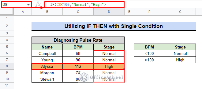
At the conclusion of the day, we can say that Alyssa is the only patient with high blood pressure, and everyone else has normal BP.
Read More: How to Use IF Condition Between Two Numbers in Google Sheets
2. Using AND/OR Criteria
Since the IF THEN formula primarily performs a logical test with TRUE and FALSE outcomes, we can further enrich the criteria by integrating the AND and OR logical conditions into the formula. We are then able to conduct an initial test using multiple criteria.
2.1 IF THEN with AND Criteria
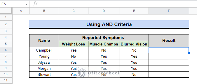
Let’s say we have a dataset of patients who have symptoms that can be used to determine if they have Nephropathic diabetes or Normal diabetes. Damage to the kidney occurs in patients with nephropathic diabetes. Loss of weight, Muscle cramps, and blurred vision are common symptoms.
Steps:
- First, we must choose a cell, F6.
- Now we may say that the patient has nephropathic diabetes if they have checked Yes to all the conditions, including weight loss, muscle cramps, and blurred vision.
- To determine the outcome, we’ll utilize the formula below.
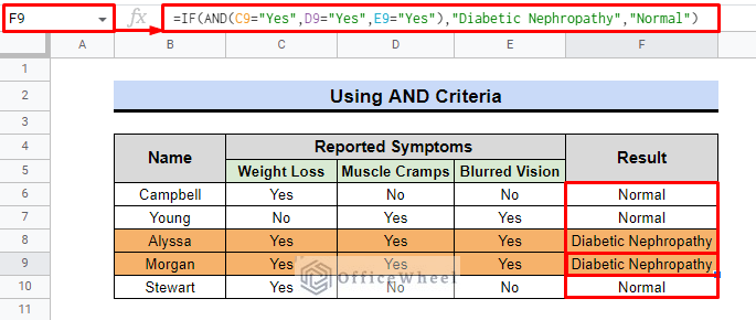
=IF(AND(C6="Yes",D6="Yes",E6="Yes"),"Diabetic Nephropathy","Normal")- Finally, press ENTER to see the findings.
Formula Breakdown:
- (C6=”Yes”,D6=”Yes”,E6=”Yes”) as to determine whether the cell values are equal to Yes or not.
- If all the conditions are met, the AND function will perform the logical test and return TRUE if all values are Yes; otherwise, it will return FALSE.
- “Diabetic Nephropathy” will be the result if the value is TRUE.
- If the AND function returns a FALSE value then it will be “Normal”.
We discover that just two of our patients, Alyssa and Morgan, meet the requirements, thus we can deduce that they have diabetic nephropathy.
Read More: How to Use AND Function in Google Sheets (4 Useful Examples)
2.2 IF THEN with OR Criteria
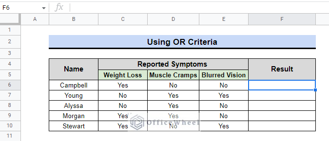
There is a different form of diabetes called Diabetic Retinopathy, which affects the blood vessels in the eyes. Patients with blurred vision frequently have this condition. Those who do not lose weight, however, stand the risk of developing diabetic retinopathy.
Steps:
- Again, we must begin by selecting cell F6.
- To rule out all the patients having diabetic retinopathy, we can utilize the OR criterion since they must declare either a No for weight loss or a Yes for blurred vision.
- Therefore, we are going to use the following formula.
=IF(OR(C6="No",E6="Yes"),"Diabetic Retinopathy","Normal")- Click ENTER at the end to view the outcome.

Formula Breakdown:
- The IF function executes the logical test using the OR function to satisfy the OR criterion of our objective.
- OR(C6=”No”,E6=”Yes”), here, OR criterion validates the arguments. If any of the parameters examined by OR are TRUE, it will return TRUE; If all parameters are FALSE, it will display a FALSE value.
- If the value is TRUE, then it will return “Diabetic Retinopathy”.
- “Normal” refers to the false value returned by the OR criterion.
We can see that, of the five individuals, three are either at risk for or have already developed diabetic retinopathy.
Read More: How to Use IF and OR Formula in Google Sheets (2 Examples)
Similar Readings
- How to Highlight Row If Cell Is Not Empty in Google Sheets
- Google Sheets: Conditional Formatting Row Based on Cell
- How to Use ARRAYFORMULA with IF Function in Google Sheets
- Use REGEXMATCH Function for Multiple Criteria in Google Sheets
- How to Use VLOOKUP for Conditional Formatting in Google Sheets
3. Applying Nested Conditions
Although applying many conditions at once when using multiple IF statements in Google Sheets may seem complicated, it makes the process much simpler. Consider the following example.
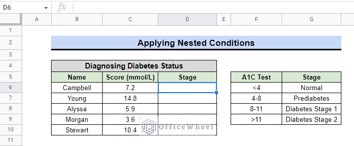
Assume we have a dataset of a few patients that includes their most recent A1C Test results to check for diabetes. We must assess the level of diabetes they have. We can do this by nesting multiple IF functions inside one another to cover all given conditions.
Steps:
- Select cell D6 first.
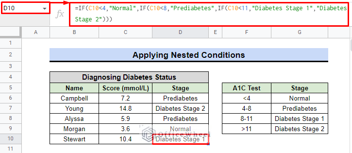
- The formula that we’ll employ is as follows:
=IF(C6<4,"Normal",IF(C6<8,"Prediabetes",IF(C6<11,"Diabetes Stage 1","Diabetes Stage 2")))- Finally, press ENTER to learn the outcome.
Formula Breakdown:
- The IF function will test C6<4 as the first logical input.
- “Normal” is the value to display if the first argument returns TRUE.
- If the first logical argument returned FALSE, the IF function will verify the second logical argument, which is C6<8.
- It will display “Prediabetes” If the second parameter is TRUE.
- If the second argument is FALSE, the third argument to test is C6<11.
- It will output “Diabetes Stage 1” If the third logical argument is TRUE.
- If the third logical statement is FALSE then it will display “Diabetes Stage 2”.
We can see that the formula identified their level of diabetes based on the result of their test. Stewart, for instance, has Diabetes Stage 1 since his score is between 8 and 11.
Read More: How to Use Nested IF Statements in Google Sheets (3 Examples)
Final Words
You can also apply conditional formatting with the IF then function. This article made an effort to address every aspect of using IF THEN in Google Sheets. For more details, visit our website OfficeWheel or leave a comment below if you have any questions about the Google Sheets if-then formula.
Related Articles
- How to Use Nested IF Function in Google Sheets (4 Helpful Ways)
- Conditional Formatting with Multiple Conditions Using Custom Formulas in Google Sheets
- Filter Values that Contains Multiple Text Criteria in Google Sheets (2 Easy Ways)
- If Cell Contains Text Then Return Value in Another Cell in Google Sheets
- Highlight Row Based on Date in Google Sheets (2 Suitable Ways)
- Match Multiple Values in Google Sheets (An Easy Guide)