Today we will look at how we can use conditional formatting with custom formula in Google Sheets.
Let’s get started.
Basics of Using Custom Formula in Conditional Formatting
We start by opening the Conditional formatting options window in Google Sheets. We do this by navigating down the Format tab to reach the Conditional formatting option.
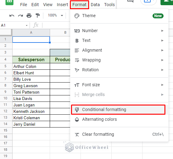
This should open the Conditional format rules tray on the right-hand side of the window.
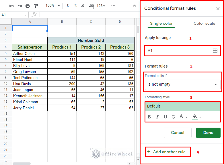
Here, we have four options to note:
- Apply to range: If you have not already selected the formatting range before opening this window or you just want to change the effect range, you can do so here.
- Format cells if…: This is our primary condition input spot. This is where we apply the various conditions for formatting, including Custom formulas.
- Formatting style: This section determines how you want your formatting to look.
- Add another rule: This allows you to add another, but a separate, condition.
Our focus will be on point number 2, the Format cells if option.
Here, in the drop-down options of Format cells if, navigate to the bottom and you will find the Custom formula is option.
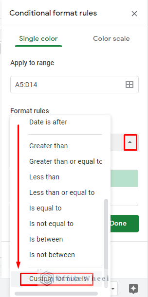
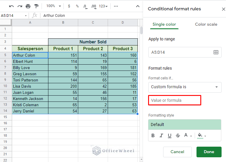
This will open an input field where you can apply your formulas.
The rest of the article sees us using various practical examples to show off how we can use custom formulas in conditional formatting in Google Sheets.
Examples of Using Custom Formula in Conditional Formatting
1. Highlight Blank Cells
Having blank cells in a large dataset can easily be missed while scrolling through it. Or highlighting true blank cells from cells with invisible values, like apostrophes (‘) and whitespaces, can also be helpful.
Our basic formula to find blank cells is:
=ISBLANK(B3)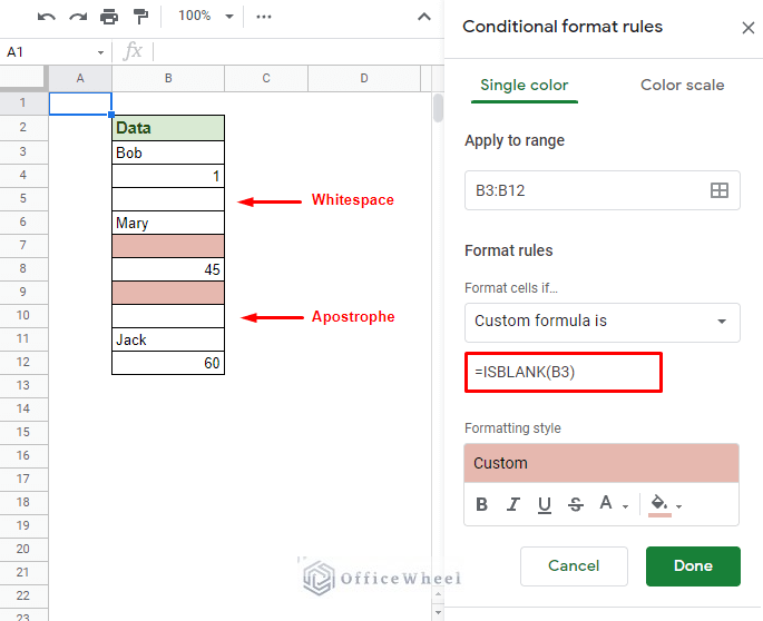
Our conditional format check starts from cell B3 and goes through the range applied in the Apply to range section, which was B3:B12 in our case.
2. Highlight Duplicates
The next common scenario where we might need to use conditional formatting is to highlight duplicate values in our dataset.
The custom formula for that is:
=COUNTIF($B$3:$B$12,B3)>1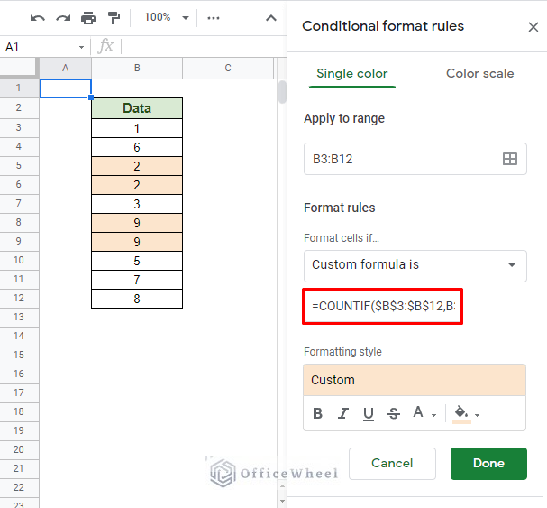
Our COUNTIF formula counts each occurrence of data down the range. With the condition “>1” the output returns either Boolean TRUE or FALSE. If TRUE, the cell is highlighted.
For a more in-depth breakdown of the formula and other iterations of it, please see our Highlight Duplicates in Google Sheets article.
3. Highlight Alternating Rows
In many cases, professional reports are printed with tables with rows highlighted alternatively. An easy way to get this done for a larger table is by using conditional formatting.
The custom formula for highlighting alternate rows in Google Sheets with conditional formatting is:
=MOD(ROW(),2)=1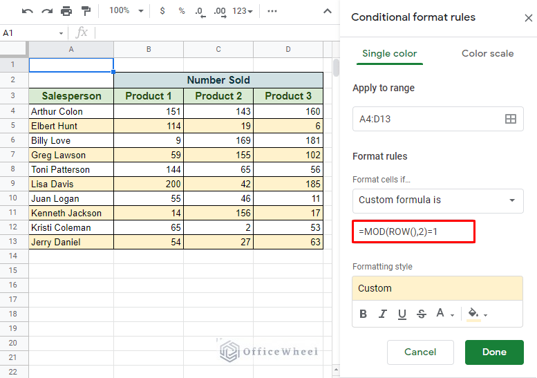
The MOD function divides the number (row number) returned by the ROW function to give us the remainder. When the remainder is 1 (meaning odd-numbered rows), the condition output is TRUE and thus the row is highlighted.
To highlight even numbered rows, use this formula:
=MOD(ROW(),2)=0The condition for even rows is that the remainder must be 0.
4. Highlight Errors
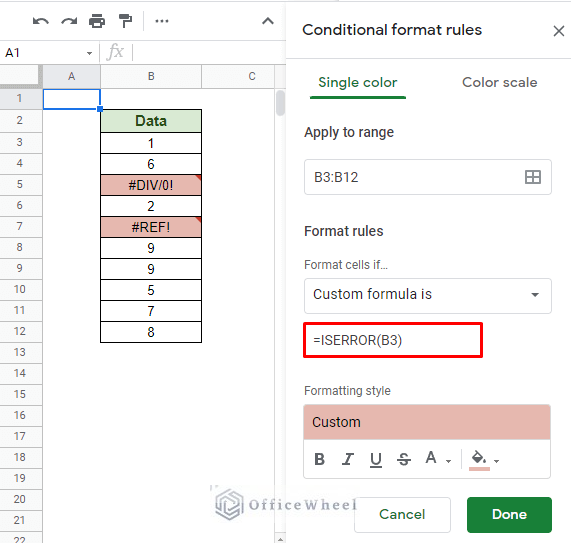
The ISERROR function comes in handy when locating errors within a dataset. But using it within the worksheet is inefficient when the dataset is large or organized in a certain way.
Even so, this function is perfect when utilized as a custom formula for conditional formatting to highlight all errors within a range.
5. Highlight Cells Based on the Value of Another Cell
One of the more important reasons to use conditional formatting in Google Sheets is to highlight cells based on the value of another cell.
From the following dataset, we will look to highlight all the cells that have a value greater than 100. The condition is placed in cell C16.
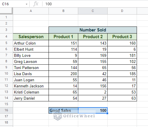
We will use the value in cell C16 in our custom formula:
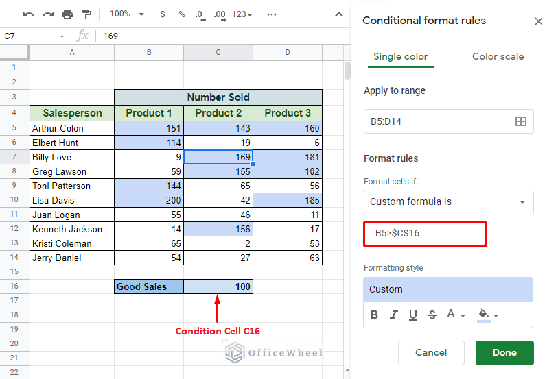
We use absolutes ($) around our condition to keep the reference in place as the formula goes ever the application range.
For a more in-depth guide, please check out our Conditional Formatting Based on Another Cell in Google Sheets article.
6. Highlight Whole Row
Another important use of conditional formatting is to highlight entire rows of data according to a given condition. Conditional formatting, by default, only highlights cells. But with the help of custom formulas, we can highlight an entire row for a single condition.
For example, we want to highlight rows from the following table that contain entries with Sales amounts less than 200.
Our formula:
=$C3<200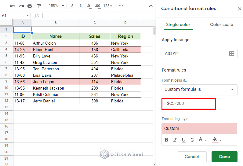
Notice that the cell that we have used to check the condition, cell C3, has its column number locked. This mixed cell reference helps set up the primary condition to highlight the entire row, as the row number is unlocked and free to move.
For more approaches and breakdown of different conditions, please check our Change Row Color Based on Cell Value in Google Sheets article.
Final Words
The use of conditional formatting with custom formulas In Google Sheets is virtually endless. What we have discussed and presented in this article are just the fundamentals and examples to help you get started to create custom formulas of your own corresponding to the conditions of your spreadsheets.
Feel free to leave any queries or advice you might have for us in the comments section below.