Conditional Formatting Based on Another Cell in Google Sheets

Conditional formatting is a powerful tool in any spreadsheet application. It helps highlight important data in your worksheet no matter how complex the condition.

With that in mind, today we will be looking at how we can apply conditional formatting based on the value of another cell in Google Sheets.

Let’s get started.

The Primary Way to Apply Conditional Formatting Based on Another Cell in Google Sheets

Our process starts with the following dataset:

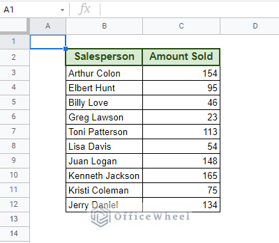
Here, we are going to be highlighting the names of the people in the Salesperson column according to their performance, which is in another cell.

Our condition for a good performance is Amount Sold > 80

Names meeting this criterion will be highlighted Green. Let’s see how it’s done.

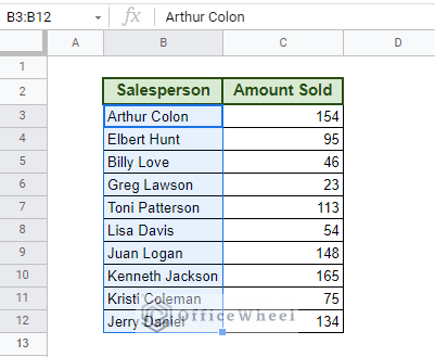
Step 1: Select the range of names. For us, it’s B3:B12.

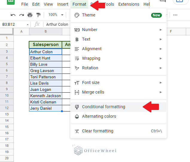
Step 2: Open the Conditional Formatting menu. Format tab > Conditional formatting

You should be presented with the Conditional format rules menu tray.

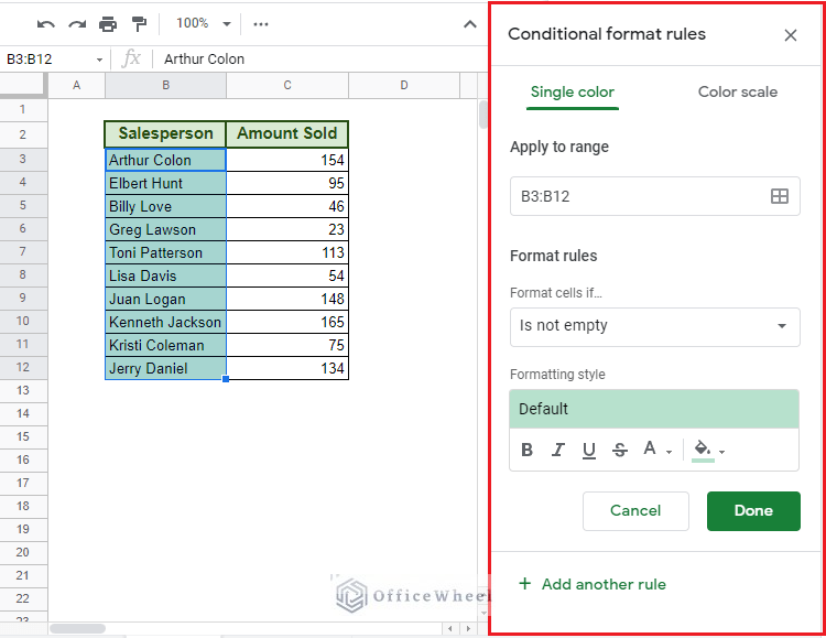
Step 3: Choose the option Custom formula is under the Format rules section.

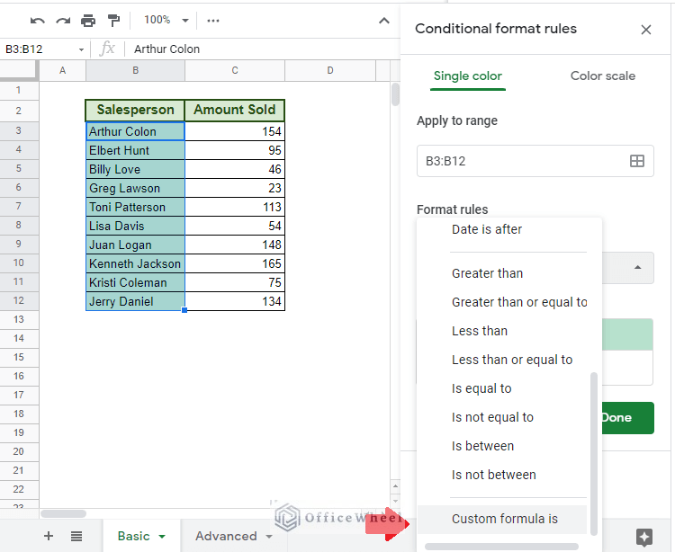
Step 4: Type in the formula for your condition:

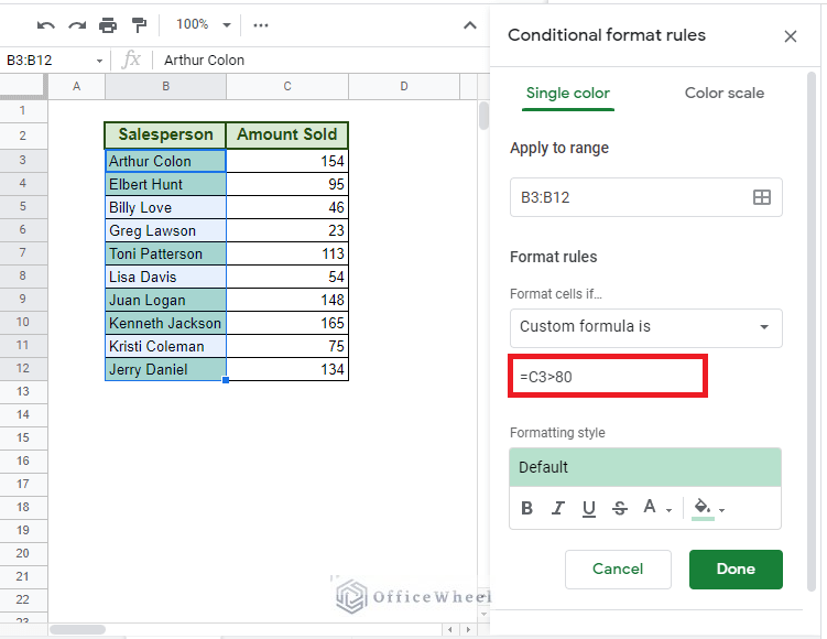
Step 5: Press Done once you are finished.

Adding Cell References to the Custom Formula for Conditional Formatting

Now, let’s put another layer to our process and make it dynamic.

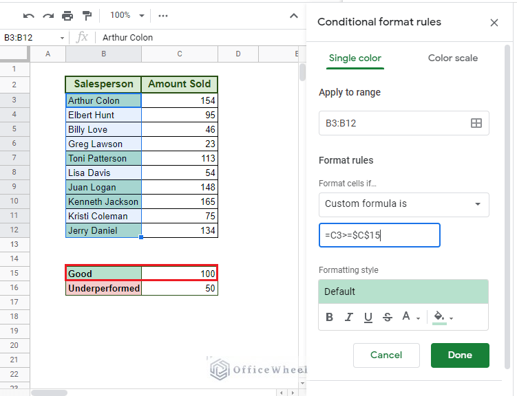
We have added a small table that gives us a reference amount to the performance, which we will be using to highlight the names.

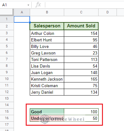
This time, instead of writing down the number in the formula, we will be using a cell reference instead.

So, let’s modify our formula a bit. Our condition this time is to highlight all the names that have sold more than 100 units with conditional formatting:

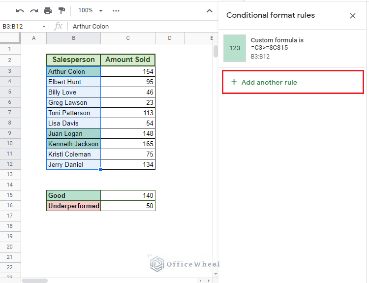
Note: We have locked our criterion cell reference

Now, if we change our criterion in our worksheet, conditional formatting will dynamically change its highlights accordingly:

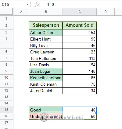
Let’s say that we also want to add the Underperformed criteria to our conditional formatting. But unfortunately, Google Sheets does not allow us to perform multiple conditional formatting at once. We can, however, add a new format to our range.

To do that, first, select the Add another rule option in the Conditional format rules menu tray.

We then add the following formula and give a different highlight, red.

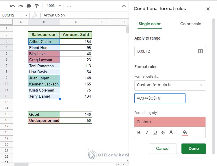
Thus we have successfully highlighted not one, but two different conditions based on the values of other cells.

Some Advanced Scenarios for Conditional Formatting in Google Sheets

Let’s now expand our dataset to match the complexity of our next processes.

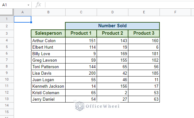
Here we have a similar dataset to the last one, but this time, we have expanded the dimension of our variable per salesperson.

1. Multiple Columns, Single Condition (OR and AND Logic)

To fully flesh out our scenario, this time, we will be looking to highlight outstanding performances in any category. And later, we are also going to be highlighting those who have been performing poorly constantly.

For our outstanding condition, we will be looking to highlight the salesperson who has sold at least one product 160 or more times.

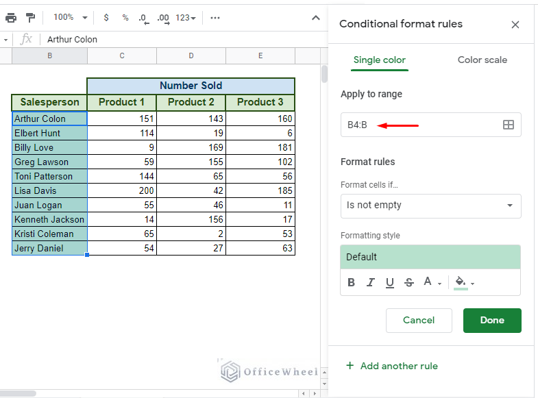
Step 1: Open the Conditional format rules menu tray. Format tab > Conditional formatting

Step 2: Input the range. To make it slightly more dynamic, we have our range as B4:B. This will make the conditional format take into account all the rows in column B starting from B4. So if you add more names to the list, the conditional format will also consider them.

Step 3: Add the custom formula:

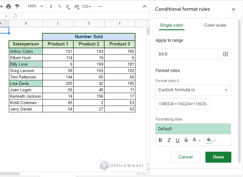
Step 4: Click Done.

We can make our formula slightly more concise by using an array version of it:

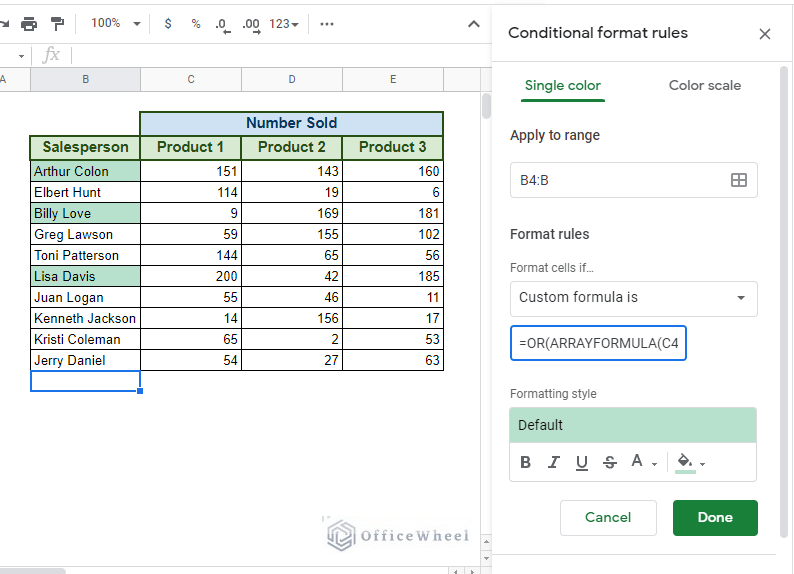
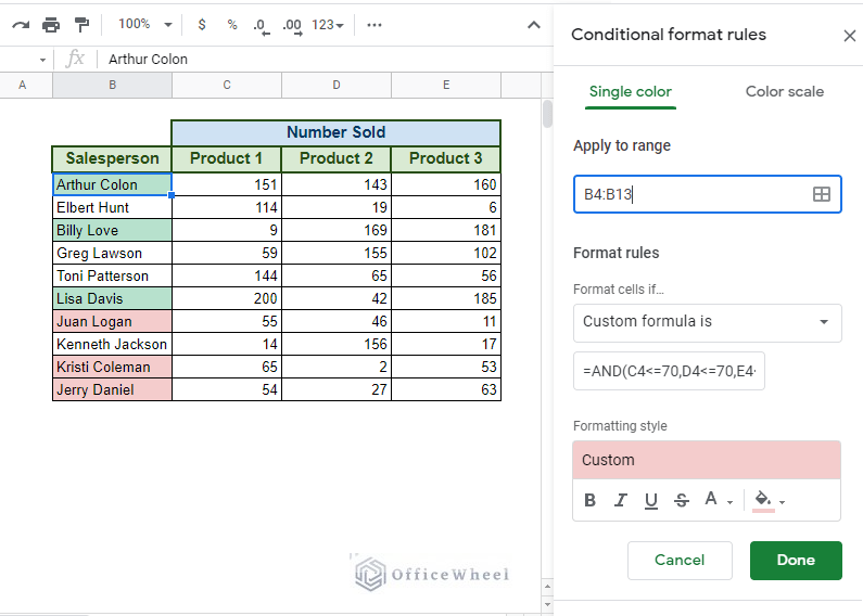
Next, we will highlight the names of the salespeople that have been consistently underperforming in all three product categories. Our numerical condition – 70 or fewer units sold for all products.

This time, we will be using the AND logic to take all three categories into account. Thus, our new formula for conditional format:

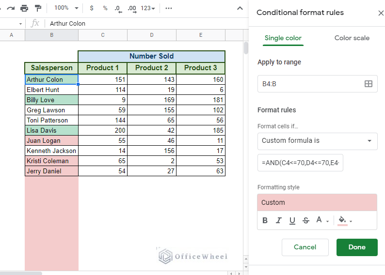
The rows beyond our table are also highlighted because of the range we have inputted, B4:B, since blank cells also mean that their value is less than 70. You can easily remedy this by limiting the range to the table, B4:B13.

A more concise version of the formula:

Congratulations! You have successfully applied conditional formatting based on the values of multiple other cells!

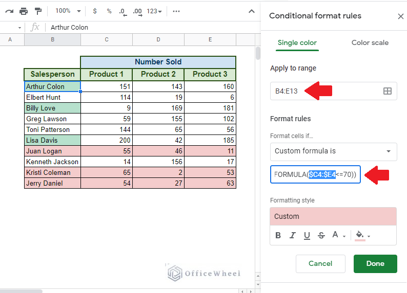
2. Applying Conditional Formatting to the Entire Row

Continuing from our previous example, we will now be applying the conditional format to not only the name column but also to the rest of the row.

Doing so might be easier than you realize. We only have to make two simple changes:

Change the range in the Apply to range section to B4:E13, so that our formatting covers the entirety of the table.

Add absolutes ($) in front of the column numbers (C, D, and E for basic formula or C and E for the array version) to lock these values down. This stops the value from moving as the formula moves.

You can, of course, apply the same steps for the other conditional formats.

Final Words

Conditional formatting in Google Sheets is fairly simple, whether it be from the immediate cell or another cell. We hope that the methods and scenarios we have discussed in this article helped you understand conditional formatting better and that you will be able to effortlessly use them for your spreadsheets.

Feel free to leave us a comment regarding any queries or advice you might have for us.

Related Articles for Reading

• Conditional Formatting with Multiple Conditions Using Custom Formulas in Google Sheets
• Highlight Duplicates in Google Sheets (4 Ways)