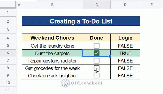
Today, we will look at how we can use Conditional Formatting with a Checkbox in Google Sheets. Conditional Formatting and Checkboxes are widely used in this application individually, but combining them both brings in a new dimension of spreadsheet customizability. In this article, we’ll see 3 suitable examples to use Checkbox with Conditional Formatting in Google Sheets with clear images and steps. At last, you’ll get an output like the below image.
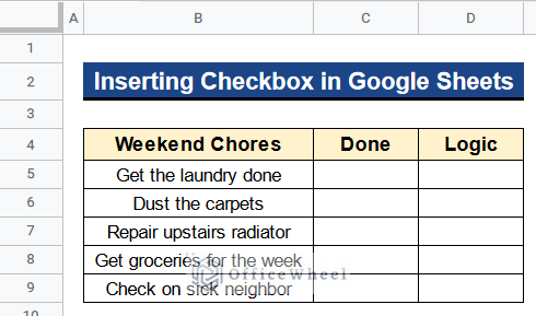
A Sample of Practice Spreadsheet
You can download Google Sheets from here and practice very quickly.
How to Insert Checkbox in Google Sheets
Let’s start with the fundamentals, that is to insert a Checkbox in Google Sheets. But if it is too trivial for you, please feel free to jump to the examples section to see how we can use Checkboxes with Conditional Formatting in Google sheets. We have the following dataset where we have some weekend chores in Column B. Now, we want to insert Checkboxes in Column C beside every chore.
Steps:
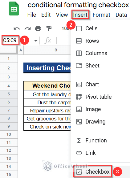
- Firstly, select the cells you want to insert the Checkbox You can also select a range of cells. Here the range is from Cell C5 to Cell C9.
- Secondly, navigate to the Insert tab and select the Checkbox option.
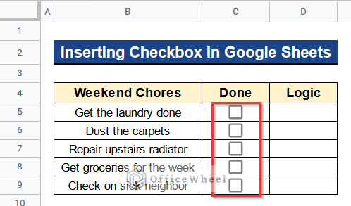
- And, you can see the Checkboxes in Column C.
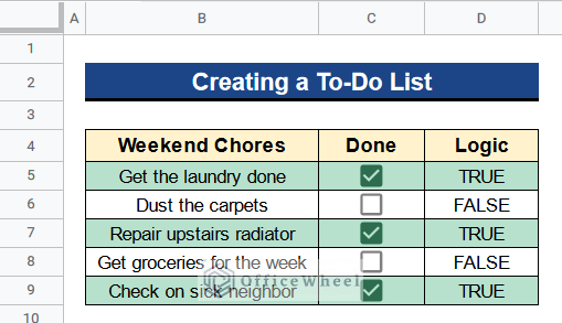
- At its base, Checkboxes are no different from Boolean outcomes of TRUE and FALSE, and Googles Sheets views them as such when operating with them. A simple check will prove this.
- Now, we will display the result of the Checkbox in Column D by writing a simple formula in Cell D5:
=C5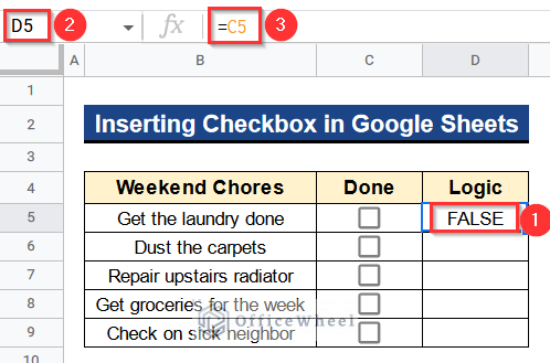
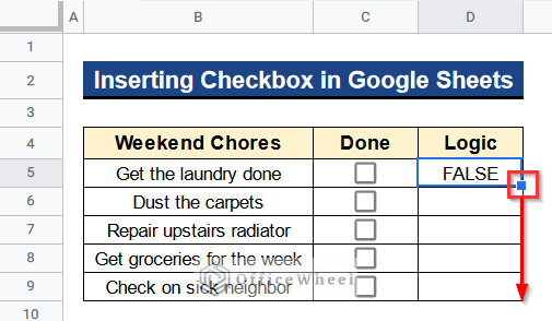
- After that, apply the Fill Handle tool to use the formula in the rest of the cells of Column D.
- Then, you’ll see the Boolean outcomes in all the cells of Column D.
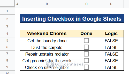
- Finally, when the box is not checked the result is FALSE and TRUE when the box is checked.
- We will use this understanding later when creating the custom formula for Conditional Formatting.
Read More: How to Copy Conditional Formatting in Google Sheets
Similar Readings
- Change Row Color Based on Cell Value in Google Sheets (4 Ways)
- How to Reset Checkboxes Daily in Google Sheets (2 Methods)
- Use COUNTIF Function to Count Checkbox in Google Sheets
- How to Filter with Checkboxes in Google Sheets (4 Ideal Examples)
3 Suitable Examples to Use Conditional Formatting with Checkbox in Google Sheets
Below we’ll see 3 suitable examples of how we can combine Checkboxes with Conditional Formatting for practical use in Google Sheets. We’ll use some custom formulas in all the cases.
Example 1. Creating a To-Do List
First of all we’ll create a to-do list with Checkboxes and apply Conditional Formatting there. The Conditional format rules in Google Sheets do not have any built-in conditions that directly work with Checkboxes; thus, we have to take advantage of the Custom formula is option under the Conditional Formatting menu.
Steps:
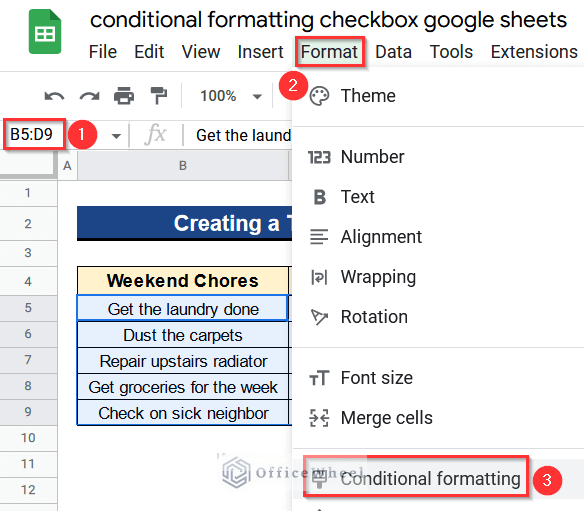
- At first, activate all the cells from Cell B5 to D9.
- Then, simply navigate to the Format tab and select the Conditional Formatting option.
- Here, in the Conditional format rules window move to the Format rules menu.
- Next, in the Format cells if… drop-down list, find the Custom formula is option at the bottom.
- After that, to highlight the entire row with our primary condition being the Checkbox, we enter the following custom formula:
=$C5- Consequently, you can choose your own formatting style. We pick the green color to format our dataset.
- Then, press the Done button.
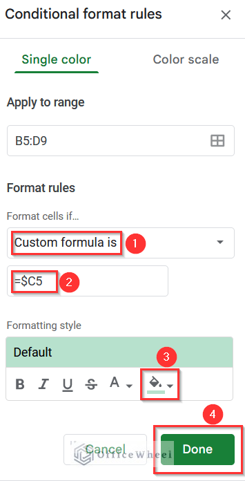
- Further, you’ll see the to-do list with Checkboxes is ready.
- In the end, when you check the box, the corresponding row will highlight with green color.

Read More: Google Sheets: Conditional Formatting Row Based on Cell
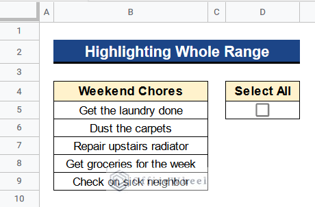
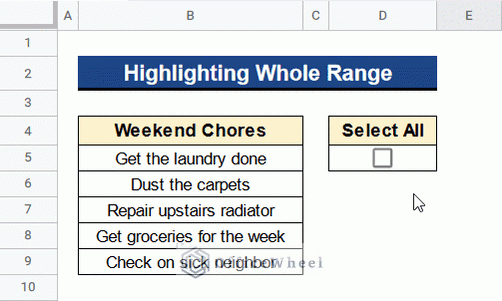
Example 2. Highlighting Whole Range
We can also define the Checkbox to highlight a range of cells at once. We only need to bring a slight change to our formula. That being, locking the cell reference of the Checkbox. For our example, we will highlight all the weekend chores in Column B as soon as the box is checked.
Steps:
- First of all, select all the cells in the range from Cell B5 to B9 and go to Format > Conditional Formatting.
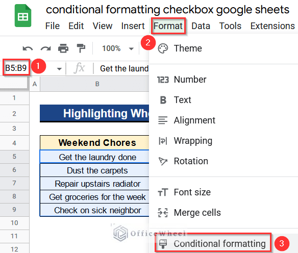
- Then, choose the Custom formula is option under the Format rules menu.
- After that, write the following custom formula in the formula box:
=$D$5- Next, choose the color green from the Color option and click the Done button.
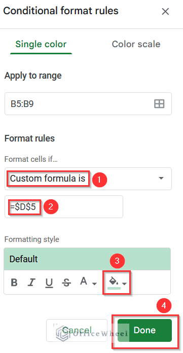
- Lastly, all the values will be highlighted in green when you check the box.
Read More: Conditional Formatting Based on Another Cell in Google Sheets
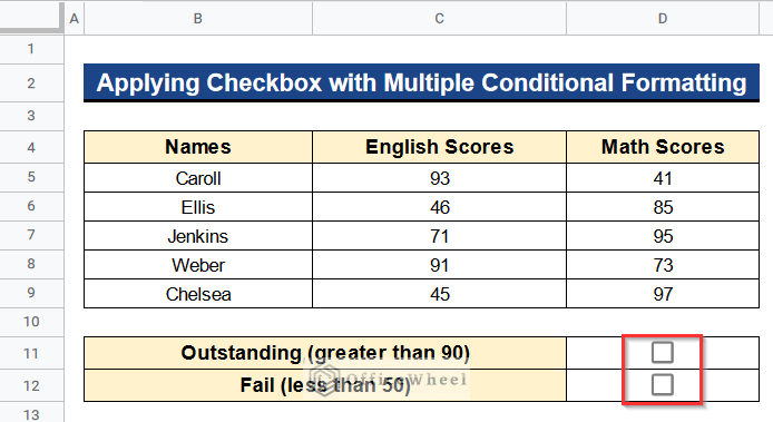
Example 3. Applying Checkbox with Multiple Conditional Formatting
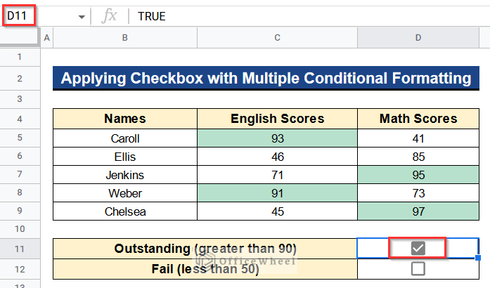
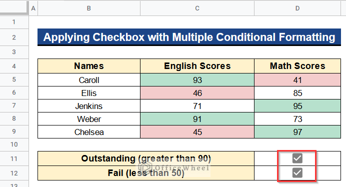
Now, we’ll apply the Checkbox with multiple Conditional Formatting. Here, we have a dataset that contains the marks obtained by some students of two different subjects in Columns C and D. Notice that we have added two Checkboxes to determine and highlight certain results. Our first condition is to highlight the cells that contain outstanding results (greater than 90) when the Checkbox is checked. Our second condition is to highlight the cells that contain failing results (less than 50) when the Checkbox is checked. For these purposes, we’ll use the AND function as the custom formula under the Conditional Formatting window. This function gives TRUE when all the conditions are TRUE and FALSE when any of the conditions is FALSE. Let’s see how it’s done.
Steps:
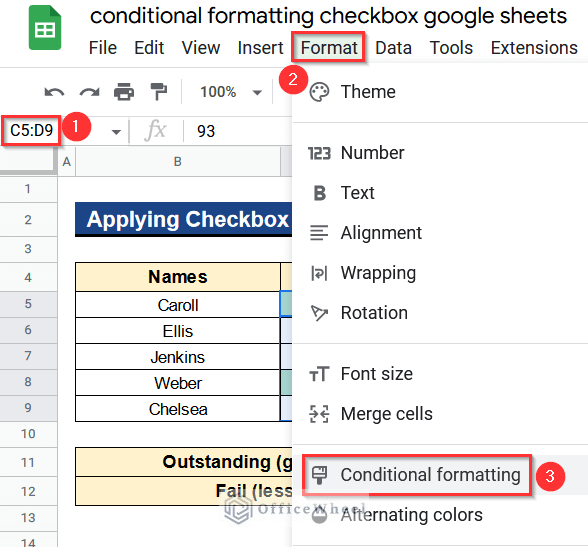
- Before all, select all of the cells in the range from Cell C5 to Cell D9, then choose Format > Conditional Formatting.
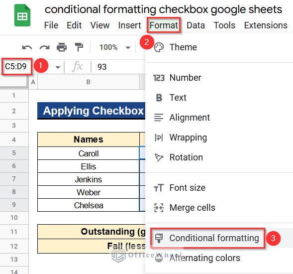
- Choose Custom formula is from the Format rules menu after that.
- Thereafter, fill out the formula box with the following unique formula:
=AND($D$11,C5>90)- Then select green from the Color button and press the Done button.
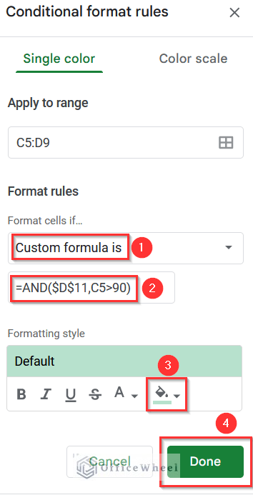
- Now, if you check Cell D11, then all the values greater than 90 of your dataset will highlight with green color.
- Again, activate all of the cells in the range from Cell C5 to Cell D9.
- Then, go to Format > Conditional Formatting.
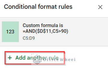
- Next, click on the Add another rule option at the bottom of the Conditional Formatting rules window to add the second condition.
- Moreover, select Custom formula is from the Format rules option.
- Then, enter the following custom formula in the formula box:
=AND($D$12,C5<50)- Next, choose pink from the Color button, and then click the Done button.
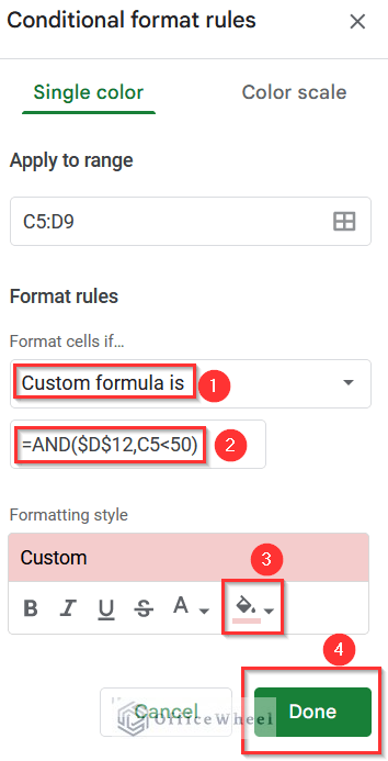
- Now if you check Cell D12, all of your dataset’s values below 50 will be highlighted in pink.
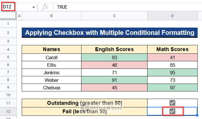
- Ultimately, all of your dataset’s values below 50 and above 90 will be highlighted in pink and green, respectively, when you check both cells.
Read More: Conditional Formatting with Multiple Conditions Using Custom Formulas in Google Sheets
Final Words
That concludes the ways we can use Conditional Formatting with Checkbox in Google Sheets. We hope our discussion comes in handy. Please feel free to leave any queries or advice you might have for us in the comments section below. You will also find different articles related to google sheets on our officewheel.com. Visit the site and explore more.
Related Articles
- Search in All Sheets in Google Sheets (An Easy Guide)
- Highlight Duplicates in Google Sheets (4 Ways)
- Pivot Table Formatting in Google Sheets (3 Easy Ways)
- Copy Formatting From One Sheet To Another In Google Sheets (2 Ways)
- Highlight Duplicates in Two Columns in Google Sheets (2 Ways)
- Google Sheets: Highlight Row If Cell Is Empty