Conditional formatting is an excellent technique for visualizing data in a spreadsheet. It has the ability to swiftly highlight critical information. Besides that, the VLOOKUP function is a lookup function for locating matching rows in a table or range. In this article, I will demonstrate 5 simple examples of using the VLOOKUP function for conditional formatting in Google Sheets.
5 Simple Examples to Use VLOOKUP Function for Conditional Formatting in Google Sheets
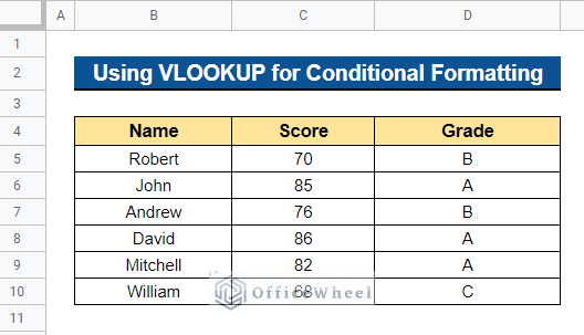
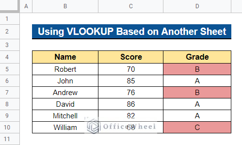
We will use the dataset below to demonstrate the examples of using the VLOOKUP function for conditional formatting in Google Sheets. The dataset contains student scores and grades. Here, we will use the VLOOKUP function for conditional formatting in Google Sheets to visualize the students’ grades.
1. Applying for Less than Condition
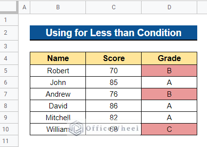
We want to highlight the student’s grades who got less than 80 marks on the exam. We can easily accomplish this using the VLOOKUP function for conditional formatting in Google Sheets.
Steps:
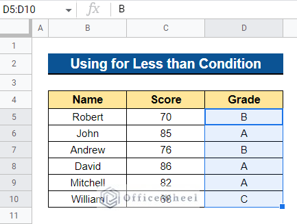
- First, select all the cells where you want to apply the conditional formatting in Google Sheets. In our case, we selected Cell D5:D10.
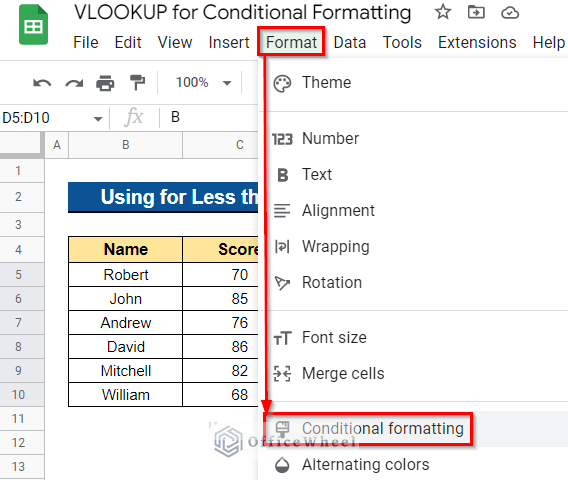
- Now, go to the Format tool from the top menu bar and select Conditional formatting.
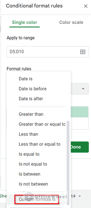
- It will open the Conditional format rules dialog box. Now, click on the drop-down icon on the Format cells if…
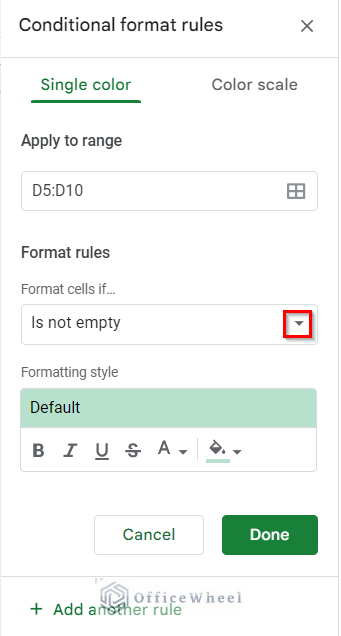
- Then, choose the Custom formula is option from the Format cells if…
- Now type the formula below in the Values In addition, you may wish to customize the formatting style. Click on the drop-down image icon to choose a color for highlighting.
=VLOOKUP($B5,$B$5:$C$10,2,FALSE)<80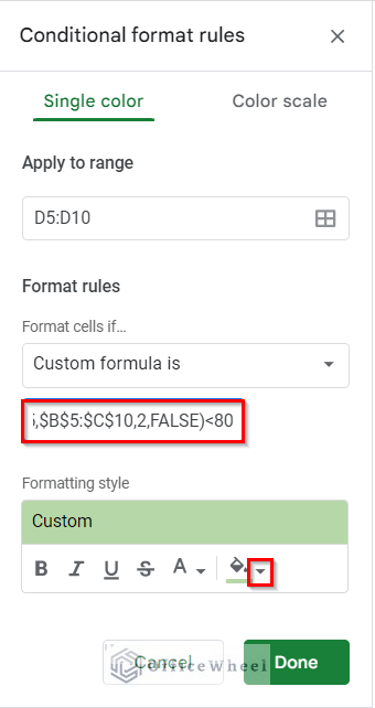
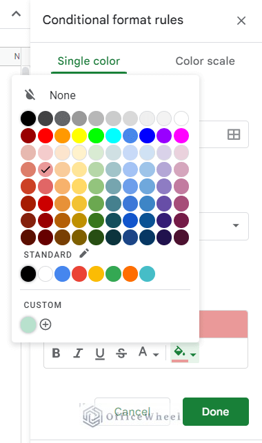
- Choose a color to highlight your results.
- Now, all the grades that are less than 80 marks are highlighted.
Read More: Google Sheets: Conditional Formatting with Multiple Conditions
2. Using for Greater than Condition
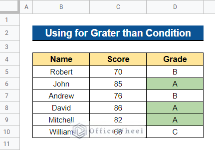
We wish to highlight the students’ grades who received 80 or more on the exam. We can easily achieve this in Google Sheets by utilizing the VLOOKUP function for conditional formatting.
Steps:
- First, follow the first 4 steps from the previous method. Now, type the following formula in the Values option and choose your desired color to highlight the results from the Formatting style image icon option.
=VLOOKUP($B5,$B$5:$C$10,2,FALSE)>=80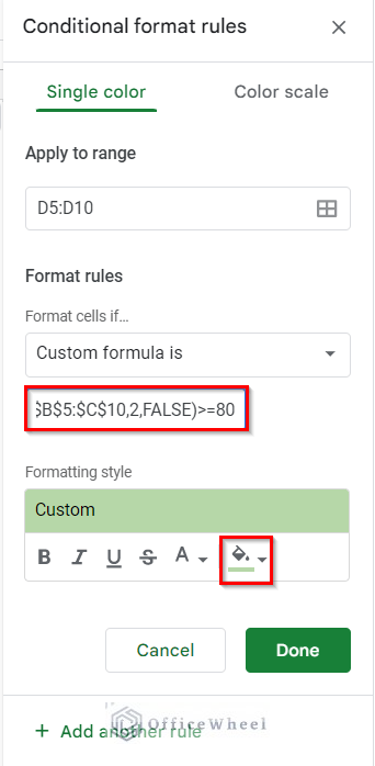
- Now, all the students who have achieved 80 or more on the exam are highlighted.
Read More: Conditional Formatting with Multiple Conditions Using Custom Formulas in Google Sheets
3. Inserting for Between Two Values Condition
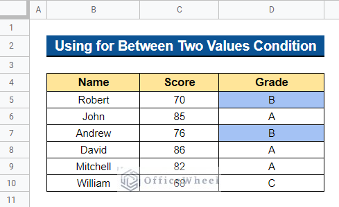
In Google Sheets, we can also utilize the VLOOKUP function for the between two values condition. For example, we wish to highlight the grades of students who received a Grade B on the exam, which indicates they received more than or equal to 70 points but less than 80 points. We will use the AND function to do so.
Steps:
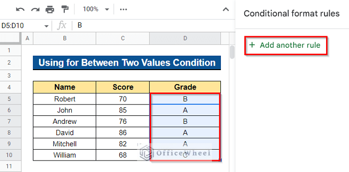
- First, select all the cells where you want to apply the conditional formatting. We selected Cell D5:D10. Now, go to the Add another rule option from the Conditional format rules dialog box.
- Then, from the Format cells if… option, select Custom formula is.
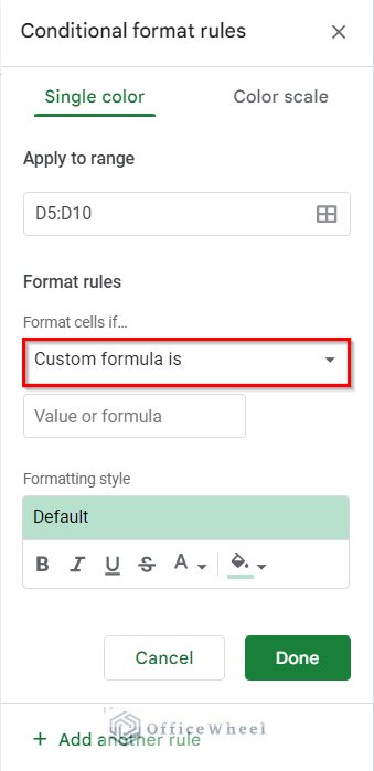
- Now, enter the formula below on the Values option and choose a color to highlight.
=AND(VLOOKUP($B5,$B$5:$C$10,2,FALSE)<80,VLOOKUP($B5,$B$5:$C$10,2,FALSE)>=70)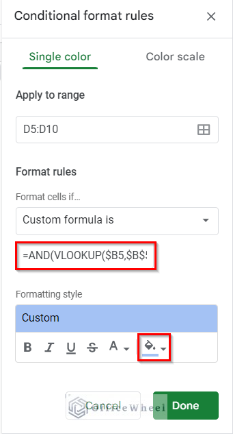
Formula Breakdown
- VLOOKUP($B5,$B$5:$C$10,2,FALSE)<80
It will show the results of those students who have earned less than 80 marks on the exam.
- VLOOKUP($B5,$B$5:$C$10,2,FALSE)>=70
It will display the results of students who received at least 70 points on the exam.
- AND(VLOOKUP($B5,$B$5:$C$10,2,FALSE)<80,VLOOKUP($B5,$B$5:$C$10,2,FALSE)>=70)
The AND function will return those cells that accept both criteria.
- You will get the desired output.
Read More: How to VLOOKUP Between Two Google Sheets (2 Ideal Examples)
Similar Readings
- Find if Date is Between Dates in Google Sheets (An Easy Guide)
- How to Concatenate with VLOOKUP in Google Sheets
- Use VLOOKUP Function with Wildcard in Google Sheets
- How to Use Multiple IF Statements in Google Sheets (5 Examples)
- Highlight Row If Cell Is Not Empty in Google Sheets
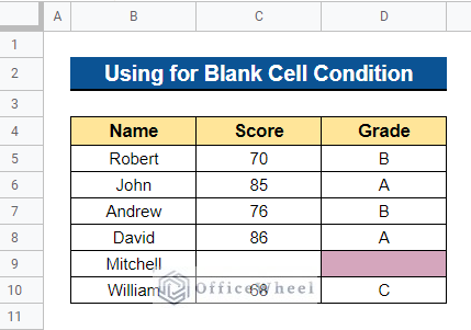
4. Employing for Blank Cell
In Google Sheets, you may have blank cells in your dataset. And you may wish to highlight the blank cells. We can do this using the VLOOKUP function in conditional formatting. We will use the ISBLANK function to do so.
Steps:
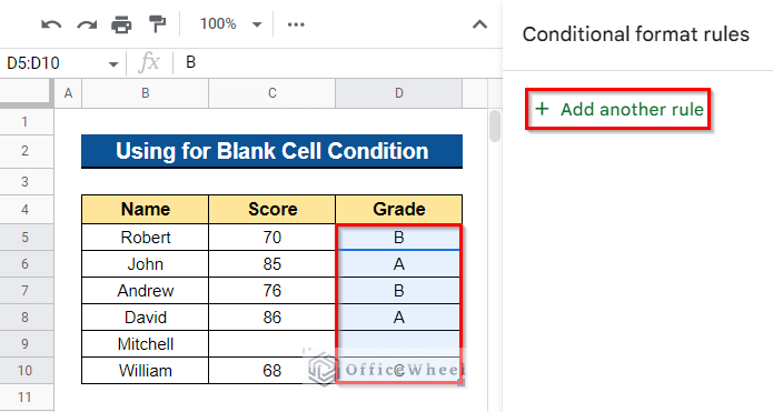
- To begin, select all the cells where you want to use conditional formatting. We chose Cell D5:D10. Now, in the Conditional format rules dialog box, select the Add another rule option.
- Now, from the Format cells if… option, choose Custom formula is. Then, type the formula below in the Values and choose a color to highlight the blank cells.
=ISBLANK(VLOOKUP($B5,$B$5:$C$10,2,FALSE))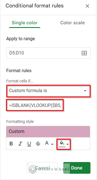
Formula Breakdown
- VLOOKUP($B5,$B$5:$C$10,2,FALSE)
It will return all the cells between Cell C5:C10.
- ISBLANK(VLOOKUP($B5,$B$5:$C$10,2,FALSE))
The ISBLANK function determines if the referred cell is empty.
- All the blank cells are now highlighted.
Read More: Highlight Cell If Value Exists in Another Column in Google Sheets
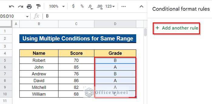
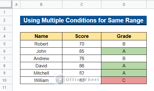
5. Using Multiple Conditions for Same Range
In Google Sheets, we could want to utilize multiple conditions for the same range. For example, we would want to highlight the grades of students who earned a Grade A on the test, indicating that they scored more than or equal to 80 points, as well as the grades of students who obtained a Grade C on the exam, indicating that they received fewer than 70 points.
Steps:
- To begin, pick all the cells where conditional formatting will be used. We chose Cell D5:D10. Select the Add another rule option in the Conditional format rules dialog box.
- Now select Custom formula is from the Format cells if… Then, in the Values section, enter the formula below and select a color to highlight the results that are less than 70 points.
=VLOOKUP($B5,$B$5:$C$10,2,FALSE)<70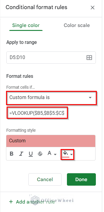
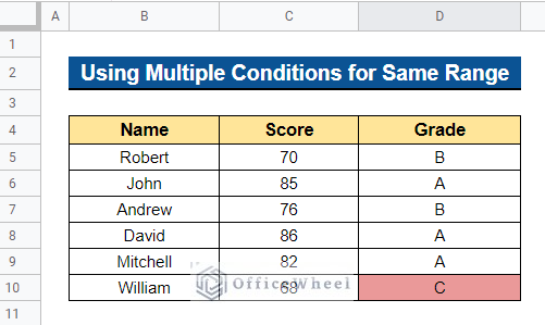
- All the students who have achieved Grade C are now highlighted in radish color.
- Now, right below the conditional format rule of the chosen cells, you’ll see an option called Add another rule.
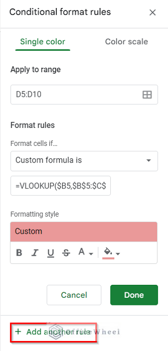
- Then, in the Values area, enter the following formula and choose a color to highlight the results that are greater than or equal to 80 points.
=VLOOKUP($B5,$B$5:$C$10,2,FALSE)>=80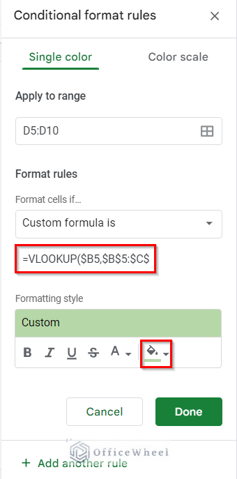
- Now, all the students who have gained Grade A are now highlighted in greenish color and all the students who have gotten Grade C are now highlighted in radish color.
Read More: Google Sheets: Conditional Formatting Row Based on Cell
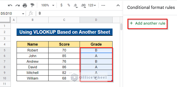
How to Use VLOOKUP Function for Conditional Formatting Based on Another Sheet in Google Sheets
Sometimes, we may wish to use the VLOOKUP function in a sheet for conditional formatting, but we want to take the data range from another sheet. We will use the INDIRECT function to do so. We can easily accomplish this by following the below steps.
Steps:
- To begin, select all the cells where you want to use conditional formatting. We picked Cell D5:D10. Select the Add another rule option in the Conditional format rules dialog box.
- Now, select Custom formula is from the Format cells if… section. Then, in the Values section, enter the formula below and select a color to highlight the results. Ensure that the sheet name and data range are enclosed by double apostrophes.
=VLOOKUP($B5,INDIRECT("Dataset!$B$5:$C$10"),2,FALSE)<80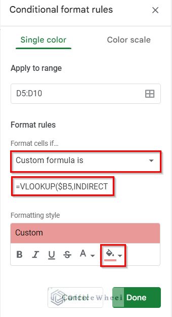
Here, we have taken the data range from the sheet named Dataset and we want to highlight those students’ grades who have earned less than 80 marks on the exam.
Formula Breakdown
- INDIRECT(“Dataset!$B$5:$C$10”)
First, the INDIRECT function will return the cell reference $B$5:$C$10 defined by the sheet called Dataset.
- VLOOKUP($B5,INDIRECT(“Dataset!$B$5:$C$10”),2,FALSE)<80
Then, the VLOOKUP function will return those students’ scores who have earned less than 80 marks on the exam.
- Thus, you will get the desired output you want.
Read More: How to VLOOKUP from Another Sheet in Google Sheets (2 Ways)
Conclusion
In this article, I have shown how to use the VLOOKUP function for conditional formatting in Google Sheets. I have shown examples of using the VLOOKUP function for less than condition, for greater than condition, for between two values condition, for blank cell condition, for multiple conditions on the same range, and for data range based on another sheet. Please feel free to ask any questions or suggest any ideas. Visit officewheel.com to explore more.
Related Articles
- How to Use VLOOKUP to Import from Another Workbook in Google Sheets
- Use Nested VLOOKUP in Google Sheets
- VLOOKUP for Partial Match in Google Sheets
- Alternative to Use VLOOKUP Function in Google Sheets
- How to Do Reverse VLOOKUP in Google Sheets (4 Useful Ways)
- Google Sheets Vlookup Dynamic Range
- How to Use VLOOKUP with Named Range in Google Sheets